
[Graphics] 3D Representation
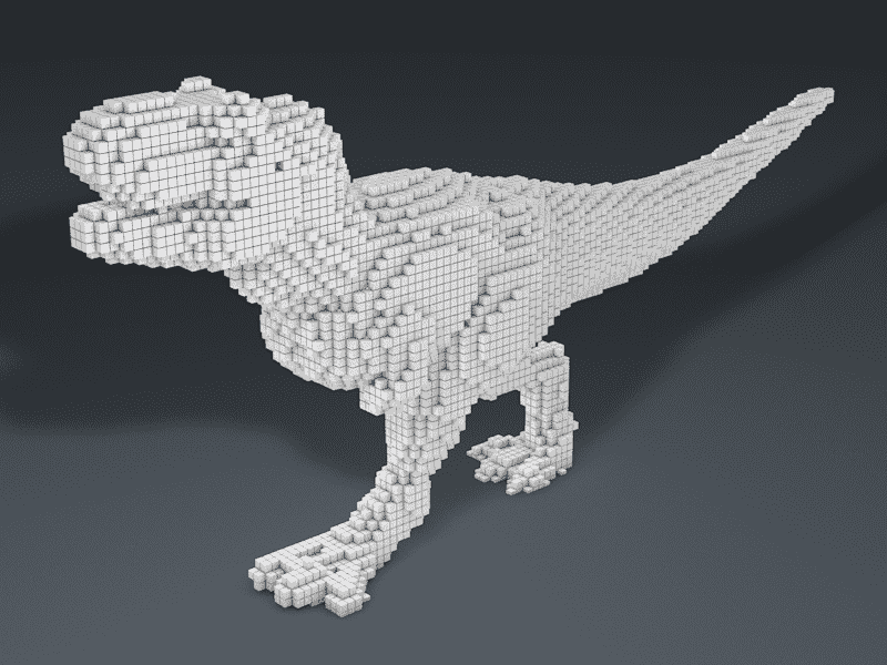
3D Grid (Voxels)
Having the regular structure like grids, for example pixels in 2D image, is key property required to apply convolution network. In that sense, we can represent 3D data as 3D grid. As with pixels in 2D case, we usually refer to grids in 3D case as voxels (volume + pixel).
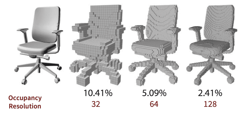
But in many applications (not all), we do not use this kind of representation, as we are typically interested in not the volume information, but surface information. For instance, when we observe the object, we cannot see the inside of that object and our vision information contains only about the surface of that.
As a result, it is a huge waste of computation since only few portion of voxels will be on the surface of objects.
3D CNNs
But actually to represent 3D data with voxels was the first idea in terms of development of neural network architectures that directly process the 3D data.
VoxNet (IROS 2015)
VoxNet, a basic 3D CNN architecture that can be applied to create fast and accurate object class detectors for 3D point cloud data. It converts 3D point cloud data (we will discuss about point cloud in the later section) collected through 3D sensors into $32 \times 32 \times 32$ volumetric occupancy grid via uniform discretization and their own occupancy model to apply CNN operations.
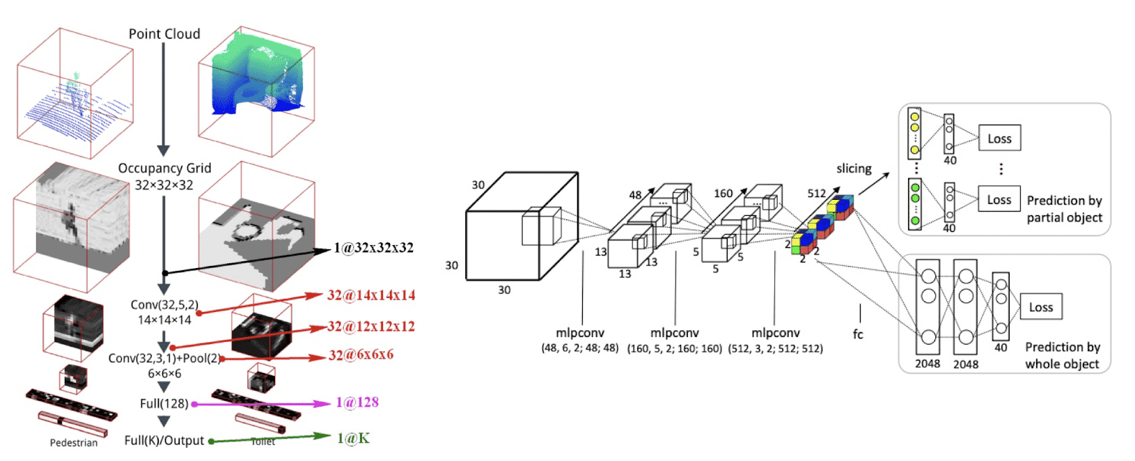
Although VoxNet achieves accuracy beyond the state-of-the-art of 3D classification, obviously it was taking a huge amount of memory and time in training. Since the memory and computation cost grow cubically as the resolution increases, these methods are not scalable for high-resolution voxels.
OctNet (CVPR 2017)
Researchers attempted to find the more efficient voxel representations that are adaptive resolution depending on the geometry information, not having uniform degree.
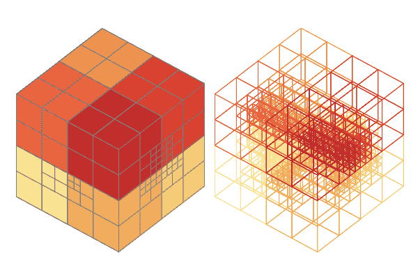
OctNet, a 3D convolutional network proposed by Riegler et al. CVPR 2017, utilized an adaptive voxel representation called octree that exploits the sparsity property of 3D data.
Suppuse a voxelized bed is given. The authors observed that the trained dense convolutional networks for 3D classification respond more strongly to voxels close to the object boundary than voxels further away.
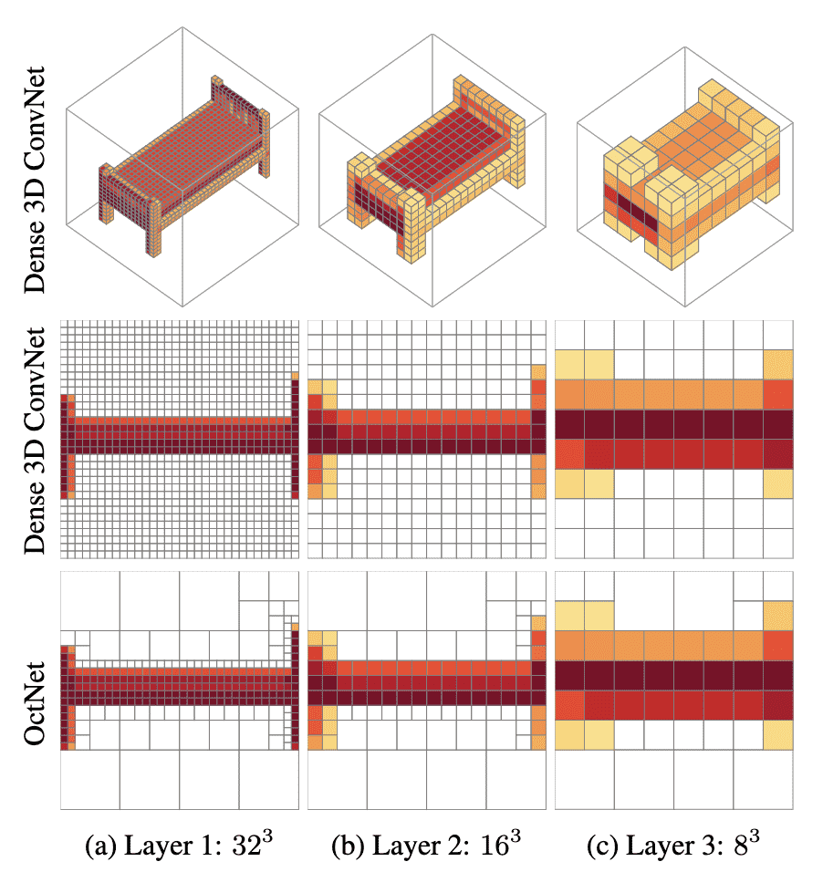
An octree partitions the 3D space by recursively subdividing it into octants. By subdividing only the cells which contain relevant information, memory for voxels can be allocated adaptively and efficiently. As a result, the region that contains object information will have high resolution, i.e. fine-grained voxels, otherwise low resolution with bigger voxels.
- O-CNN https://wang-ps.github.io/O-CNN.html https://onedrive.live.com/?authkey=%21ANNU05QdpgCE9j8&id=97002CD884825EBF%216360&cid=97002CD884825EBF&parId=root&parQt=sharedby&o=OneUp
The sort of adaptive representations including octree are obviously more efficient, but they yield some extra complexity in implementations since the 3D grid is now irregular that hampers the operation of CNN.
Multi-View Images
The straightforward way to apply 2D neural architecture to deal with 3D data might be rendering it into 2D images with multi-view.
Then, it will allow us to exploit
- data with higher resolutions than when data is represented in 3D, with identical amount of computing resources;
- massive image databases such as ImageNet via pre-trained 2D CNN.
However, there are obvious downsides:
- requires lots of images for high accuracy and thus takes lots of memory and time; (as we will see, MVCNN utilizes 80 views for their SOTA performance)
- may not be able to capture geometric details.
Multi-View CNN (ICCV 2015)
Su et al. ICCV 2015 proposed Multi-View CNN (MVCNN) that directly utilize 2D convolutional networks for 3D classification. In particular, it is trained on a fixed set of rendered multiple views of a 3D object and outperforms the state-of-the-art even only single view provided with at test time.
The framework of multi-view CNN is quite simple:
- Generate multi-views of 3D object with a rendering engine
- Compute a 2D image descriptor for each view by ImageNet pre-trained 2D CNN
-
Aggregate all descriptors and use for recognition tasks
- average
- concatenation
- voting
- etc.
Since simply averaging or concatenating separate features leads to inferior performance, the authors address the issue by learning an unified CNN to aggregate multiple views into a single compact feature for downstream tasks:
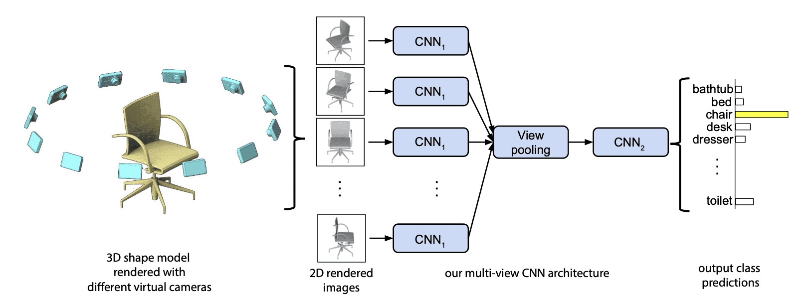
Here, each view of image feeds to the first part of MVCNN, $\text{CNN}_1$, which share the same parameters, and aggregated at a view-pooling, element-wise maximum operation across the views. Then it sent to the last part $\text{CNN}_2$ for downstream task.
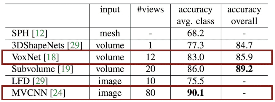
In terms of classification, this idea was effective even compared with other architecture based on 3D representation. And it gives a lesson that we don’t need to consider 3D specific architectures or represenations always for tasks with 3D data.
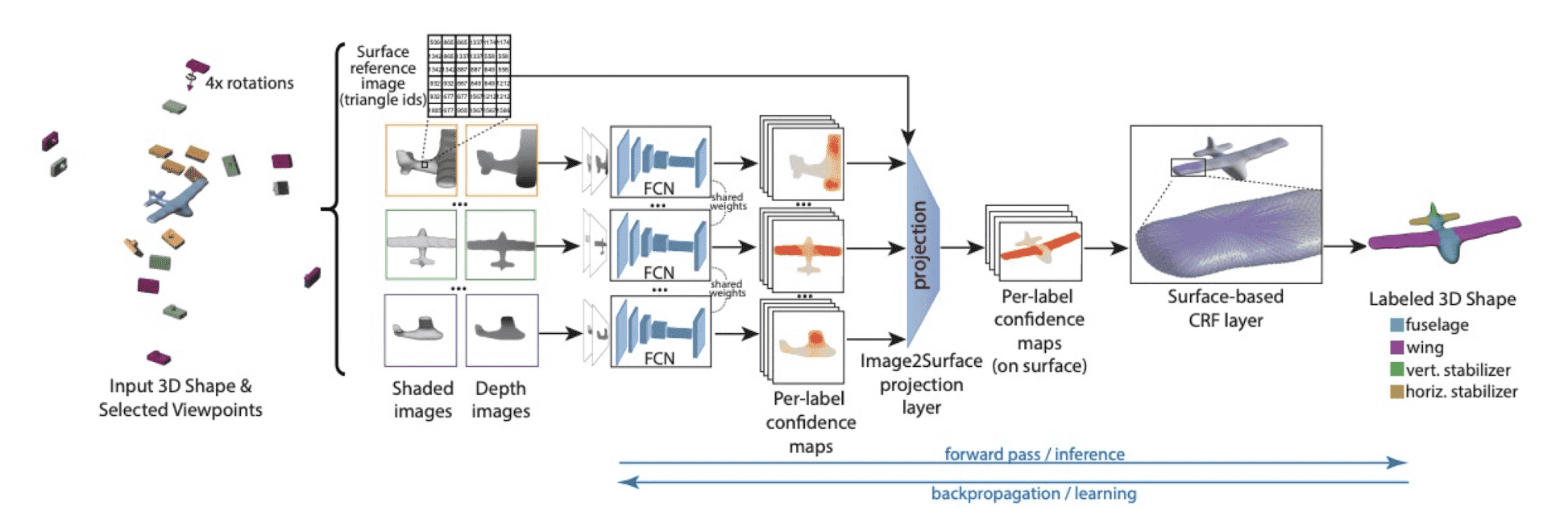
ShapePFCN (CVPR 2017)
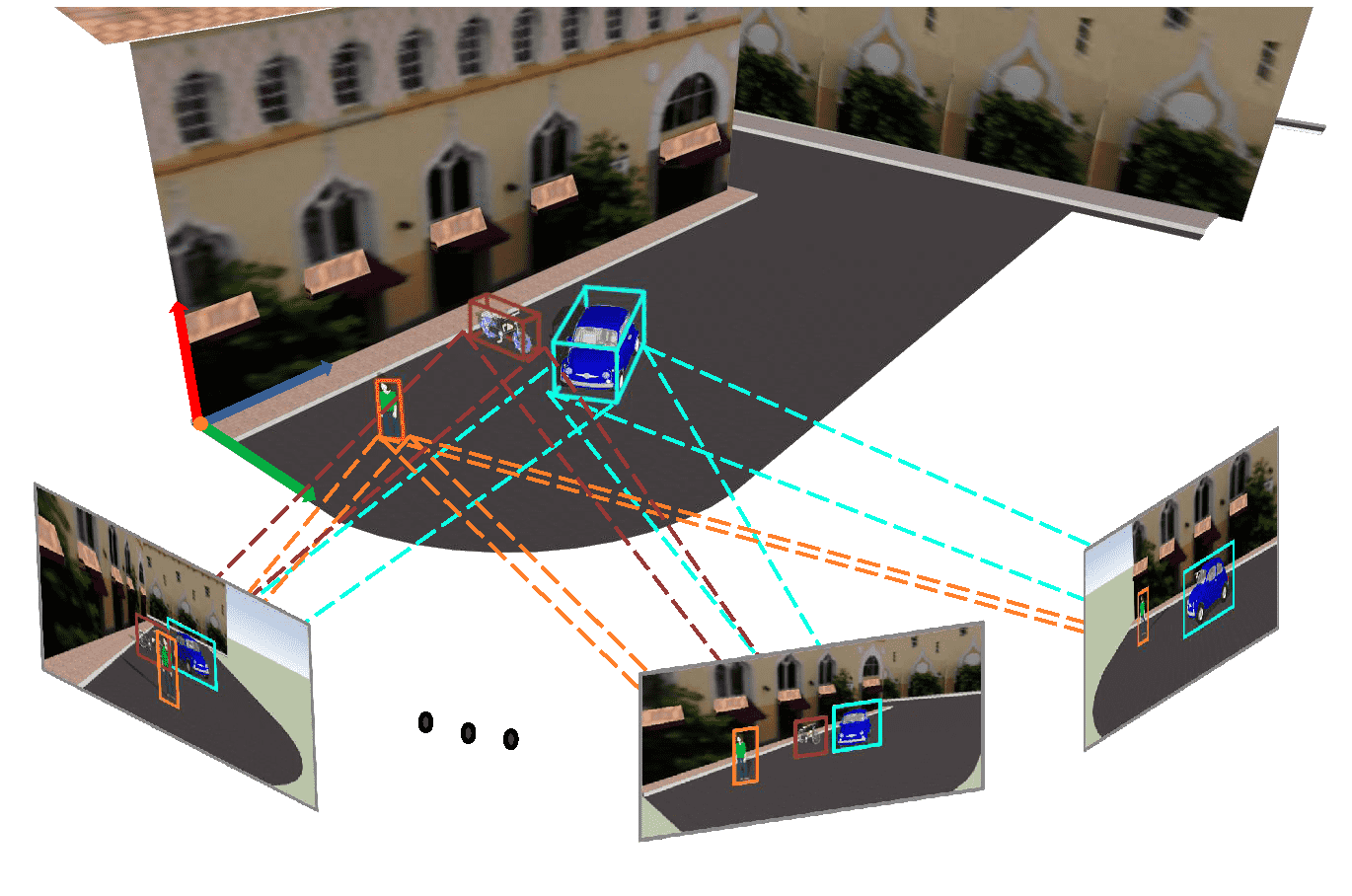
There are also some interesting techniques in the 3D segementation. ShapePFCN (Kalogerakis et al. CVPR 2017) just projects 3D data into a number of 2D images in multi-views, segments each image, and aggregates them and projects again into 3D segmentation result. For more details, please refer to the original paper!
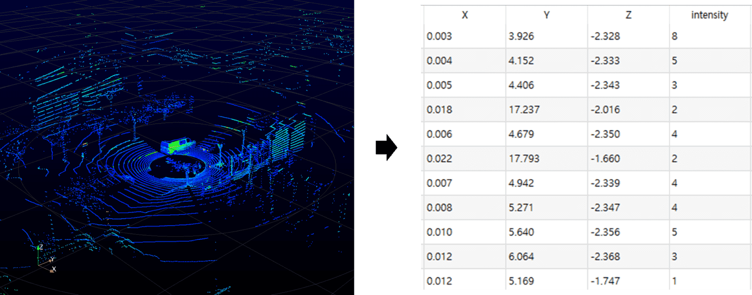
Point Cloud
Point cloud represents a 3D object in a set of only points without any connectivities. It can be considered as a collection of $(x, y, z)$ coordinates and probably we might also have some extra information such as the color information or surface normal. (We will see later how we can utilize information about it.)
Point cloud is the simplest, and common representation for many applications. For example, to my knowledge, nearly all 3D scanning devices produce point clouds.
Unlike 2D image data, point cloud data is irregular. In the case of 2D image data, information is stored in a standardized grid structure, but point cloud is stored in a way that records unordered points in 3D space. Hence, it is not usually possible to apply common deep learning techniques such as CNN, due to such an irregularity.
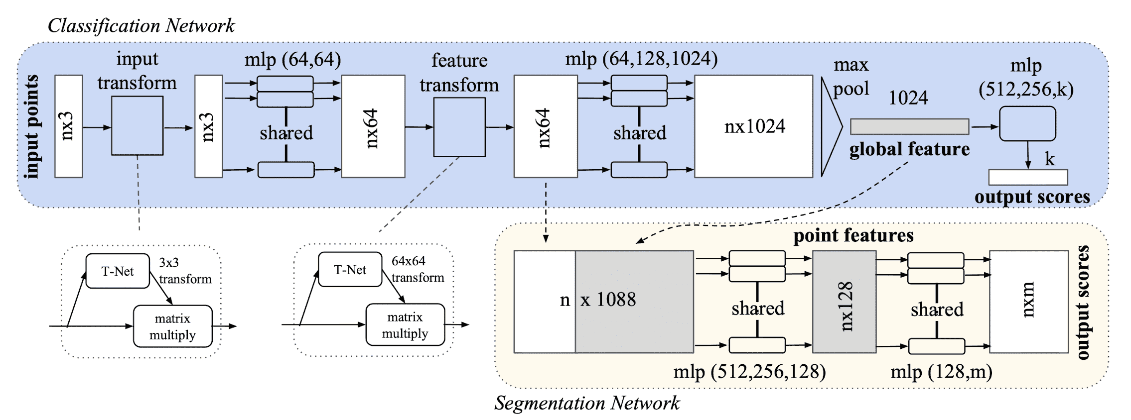
PointNet (CVPR 2017)
Thus many studies have converted point clouds into another representation such as voxel grids or image, but it was extremely inefficient and arised various issues.
Qi et al. CVPR 2017 proposed new neural architecture without any CNN for various vision tasks including classfication and segmentation, called PointNet.
The architecture of PointNet has 3 key modules, and each of them is inspired by the properties of point sets in $\mathbb{R}^n$:
-
Unordered
A network that takes a $N$ 3D point sets as an input should be invariant to $N!$ permutations
$\to$ Max Pooling Layer: Symmetric Function for Unordered Input
-
Interaction among points
Since points are not isolated and neighboring points form a meaningful subset, the model needs to capture local structures from nearby points and combinatorial interactions among local structures.
$\to$ Local and Global Information Aggregation
-
Invariance under transformations
For example, rotating and translating points all together should not modify the learned feature of the point cloud.
$\to$ Joint Alignment Network
Symmetry Function for Unordered Input
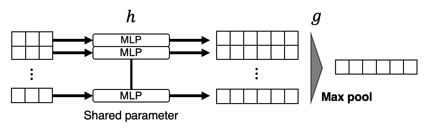
To encourage the model a permutation invariance of point set, the authors employ a simple symmetric function that takes $n$ vector as an input and outputs a new vector that is invariant to the input order.
More formally, they approximate a general function defined on a point set by applying a symmetric function on transformed elements in the set:
\[\begin{aligned} f( \{x_1, \dots, x_n \} ) \approx g(h(x_1), \dots, h(x_n)) \end{aligned}\]for $f: 2^{\mathbb{R}^{N}} \to \mathbb{R}$, $h: \mathbf{R}^N \to \mathbb{R}^K$, and a symmetric function $g: \underbrace{\mathbb{R}^K \times \cdot \times \mathbb{R}^K}_n \to \mathbb{R}$ where $h$ and $g$ are approximated by MLP network and a (column-wise) max pooling function respectively.
Local and Global Information Aggregation
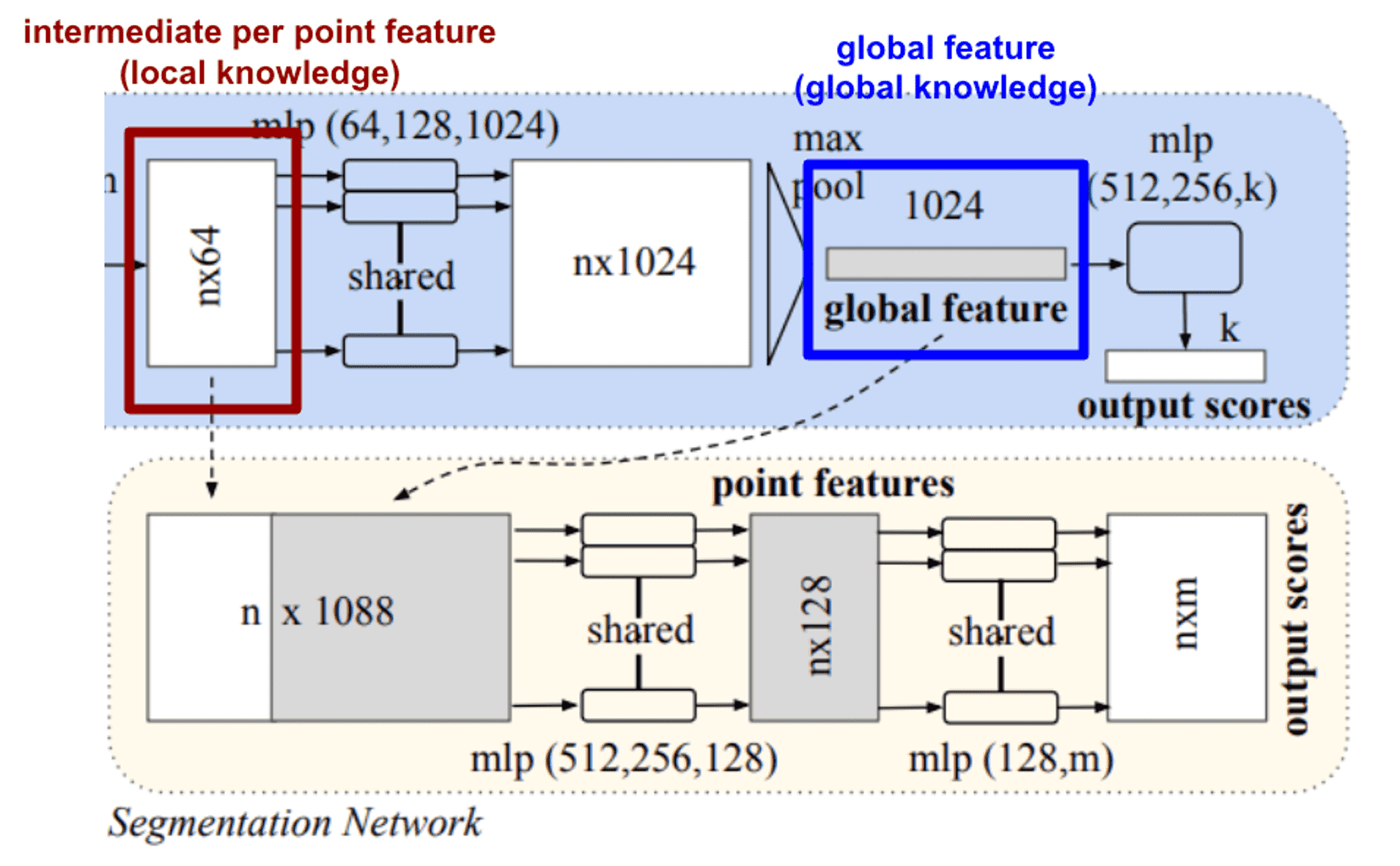
This module is designed for segmentation task.
While we can easily train an SVM or MLP classifier on the global features of shape for classification, point segmentation requires a combination of local and global knowledge for both localization accuracy and object classification.
Since the intermediate per point feature contains the local knowledge, and the global feature contains global knowledge, PointNet segmentation uses the feature that concatenates both the intermediate per point feature and the global feature, as in the figure below.
Joint Alignment Network
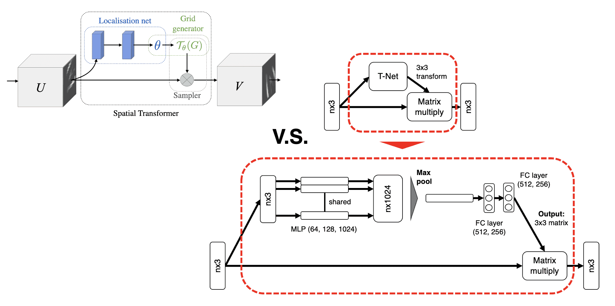
The result of both classification and segmentation should be invariant if the point cloud undergoes some geometric transformations, such as rigid body transformations.
Thus, inspired by Spatial Transformer Networks, PointNet predicts an affine transformation matrix in order for aligning all point sets to a canonical space, by a mini-network (T-net). And, it directly applies this transformation to the coordinates of input points.
And we can apply this idea into feature space to align features from different transformed input point clouds, too. However, the transformation matrix in the feature space has a much higher dimension than the spatial transform matrix, which greatly increases the difficulty of optimization. Thus authors add a regularization term to constrain the feature transformation matrix to be close to an orthogonal matrix:
\[\begin{aligned} L_{\text{reg}} = \| I - AA^\top \|_F^2 \end{aligned}\]where $A$ is the feature alignment matrix predicted by a mini-network. Note that it forces $A$ to be orthogonal. Orthogonal matrices represent transformations that preserves length of vectors and all angles between vectors, thus it is desirable to represent rigid transformation.
Summary
Due to its simplicity with outstanding performance, PointNet is one of the most popular architectures in 3D computer vision. Although PointNet addresses irregularity of point cloud, there are still downsides for point cloud representation:
-
No surface and topology information
needs to be converted to the other representation for downstream application
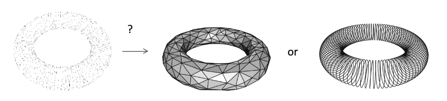
$\mathbf{Fig\ 17.}$ No topological information (source: Stanford CS348a)
-
Weak approximation power;
requires many points for the details. For instance, to approximate a circle with points, the error of piecewise linear approximation (i.e. just connecting the points) is $O(N^2)$:
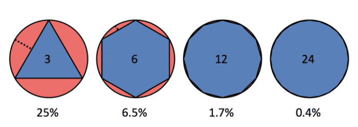
$\mathbf{Fig\ 18.}$ Piecewise linear approximation (source: Stanford CS348a)
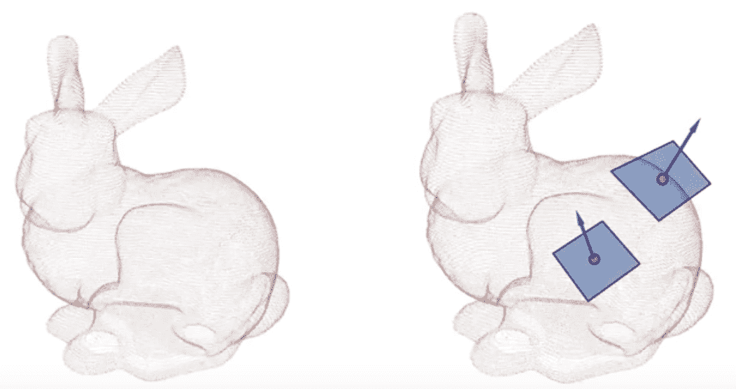
Polygon Mesh
Polygon mesh is one of the most popular representation for shapes in graphics. It represents 3D shape by a collection of vertices, edges and faces that defines the shape of a polyhedral object. And the faces usually consist of polygons including triangles, quadrilaterals, or other simple convex polygons. Hence the terminologies refer to polygon meshes depend on the type of face; for instance a triangle mesh is a special case when all the faces are triangles.
As we can see that, it is a graph-like structure (but not the same) and somewhat compact form representing surfaces since all surfaces can be defined by faces that contain surface information such as light and shadows. And especially many 3D dataset are represented as some kinds of 3D meshes.
In the context of computer graphics and 3D modeling, we often define some rules and criteria for 3D mesh to ensure that the mesh can be properly processed and rendered by computer software. And a 3D mesh that adheres to these rules is referred to as valid mesh. For example, 이거 코넬 대 주석 달자.
-
2-manifoldness
Each local region of shape should be homeomorphic (mappable) to a 2D flat plane.
-
Orientation consistency
The orientation of faces (ex. normal direction) in a mesh should be consistent. It is important for proper lighting and shading calculations.
- etc.
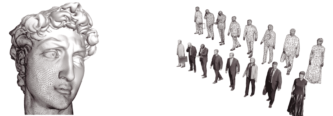
Polygonal meshes provide an efficient representation for 3D shapes and since it also captures the surface information unlike other representations, hence it shines through a variety of applications such as
But, also there are some downsides:
- (-) irregular structure
- (-) difficult to create a valid mesh
MeshCNN (SIGGRAPH 2019)
However, the non-uniformity and irregularity of mesh structure again prohibit us to exploit convolution operations.
MeshCNN ([Hnocka et al. SIGGRAPH 2019]) attempts to address this issue and designs CNN for triangular meshes by combining specialized convolution and pooling layers that operate on the mesh edges. (Hence, the edges of a mesh in MeshCNN are analogous to pixels in 2D image.) The following figure illustrates their designs for each component in MeshCNN.
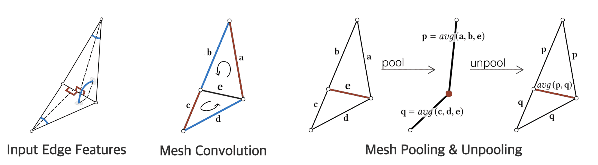
Input Edge Features
The input edge feature is a 5-dimensional vector: the dihedral angle, 2 inner angles of each adjacent face (sorted), and 2 edge ratios for each adjacent face (sorted). Note that the edge ratio is between the length of the edge and the perpendicular (dotted) line for each adjacent face.
Hence, by sorting the two face-based features and designing each vector component to be all relative, it can resolve the ordering ambiguity and ensure some invariances to translation, rotation and uniform scaling.
Mesh Convolution
Mesh version convolutional filters are applied on each edge feature vector $\mathbf{e}$, and its 4 neighboring edge features $(\mathbf{a}, \mathbf{b}, \mathbf{c}, \mathbf{d})$.
Depending on the choice of ordering of faces, there are two possible orderings: $(\mathbf{a}, \mathbf{b}, \mathbf{c}, \mathbf{d})$ and $(\mathbf{c}, \mathbf{d}, \mathbf{a}, \mathbf{b})$. (The vertices of a face are ordered counter-clockwise.) This ambiguity hampers the formation of invariance of convolutional network.
Hence, mesh convolution consists of two operations. For edge $\mathbf{e}$ and its neighbor $(\mathbf{a}, \mathbf{b}, \mathbf{c}, \mathbf{d})$, mesh convolution with kernel $\mathbf{k}$:
- Generate new features by applying simple symmetric functions on each pair to contain only relative geometric features: $$ \begin{aligned} (\mathbf{e}^1, \mathbf{e}^2, \mathbf{e}^3, \mathbf{e}^4) = ( | a-c|, a+c, |b-d|, b+d ). \end{aligned} $$
- Compute a convolution (dot product): $$ \begin{aligned} \mathbf{e} \cdot + \sum_{j=1}^4 k_j \cdot \mathbf{e}^j \end{aligned} $$
Mesh Pooling & Unpooling
And inspired by edge collapse, or interchangeably edge contraction the model can decrease the resolution of features through mesh pooling, and converse mesh unpooling:
\[\begin{aligned} & \text{pool}: (\mathbf{a}, \mathbf{b}, \mathbf{c}, \mathbf{d}, \mathbf{e}) = \left( \text{avg}(\mathbf{a}, \mathbf{b}, \mathbf{e}), \text{avg}(\mathbf{c}, \mathbf{d}, \mathbf{e}) \right) \\ & \text{unpool}: (\mathbf{p}, \mathbf{q}) = (\mathbf{p}, \mathbf{p}, \mathbf{q}, \mathbf{q}, \text{avg}(\mathbf{p}, \mathbf{q})) \end{aligned}\]Indeed, simplification of meshes by decreasing the resolution trhough edge contraction has already attempted in the early years. [14], [15]
CNN for Meshes
Likewise, various other papers have introduced modified version of CNN for meshes, such as GCNN by Masci et al. ICCV 2015, Primal-Dual Mesh CNN by Milano et al. NeurIPS 2020, and Field convolution by Mitchel et al. ICCV 2021. But they are not usually considered as common approaches.
Obivously, the implementations of them are quite complicated since they require another parameterization or specialized operations instead of the standard convolution. Also, they are verified only with a few use cases, for example MeshCNN definitely relies on good training data for a successful generalization and is fragile to adversarial remeshing attacks.
PolyGen (ICML 2020)
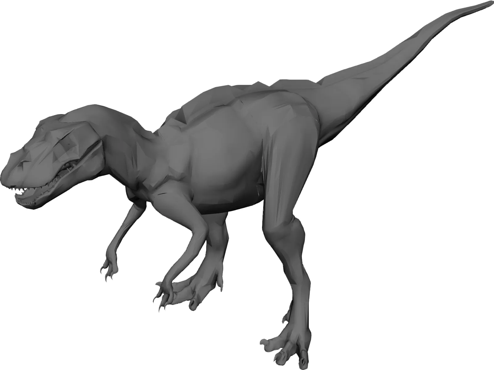
Another downside of 3D mesh is the challege of generation, since there are various complicated constraints to form a valid mesh. Also, it’s unorderness and irregularity obfuscates the generation, for example meshes that represent the same thing can have a different number of polygons even for the same set of vertices:
Due to that strain, according to Nash et al. ICML 2020, there were no existing methods that directly model mesh vertices and faces until 2020, unlike other representations such as voxels, point clouds and etc.
The first generative model that generates meshes directly, without no post-processing is PolyGen (Nash et al. ICML 2020). It is designed as an autoregressive generative model of 3D meshes, consisting of two parts implemented by Transformer: vertex model and face model. Formally, it estimates a distribution of meshes $\mathcal{M}$ which is collection of 3D vertices $\mathcal{V}$ and polygon faces $\mathcal{F}$ by chain rule:
\[\begin{aligned} p(\mathcal{M}) & = p( \mathcal{V}, \mathcal{F} ) \\ & = p (\mathcal{F} \mid \mathcal{V}) p (\mathcal{V}) \end{aligned}\]where both distribution are modeled autoregressively. For faces, we can have either triangles or generalized $n$-polygon:
\[\begin{aligned} \mathcal{F}_{\text{tri}} & = \left\{ \left( f_1^{(i)}, f_2^{(i)}, f_3^{(i)} \right) \right\}_i \\ \mathcal{F}_{\text{n-gon}} & = \left\{ \left( f_1^{(i)}, f_2^{(i)}, \dots, f_{N_i}^{(i)} \right) \right\}_i \\ \end{aligned}\]where $N_i$ is the number of faces in the $i$-th polygon. (They have a variable number of vertices)
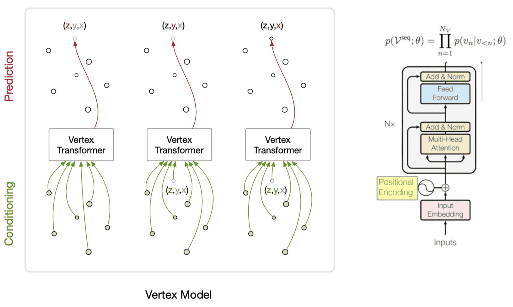
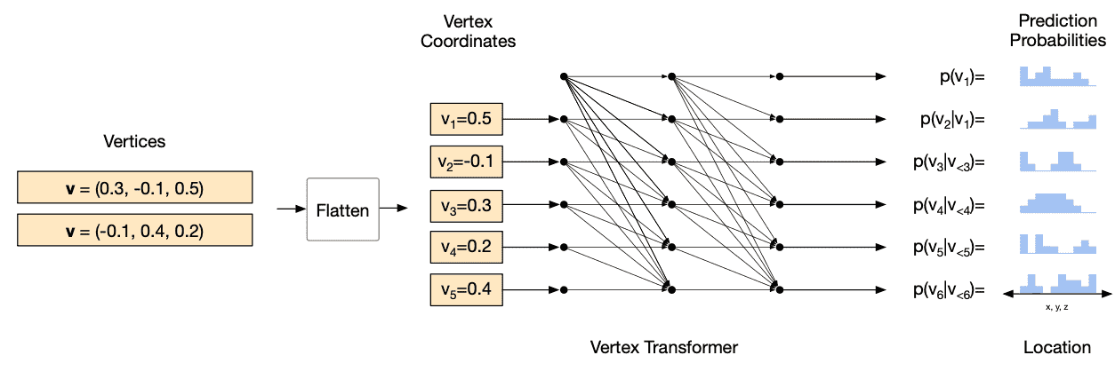
Vertex model
We model the joint distribution of vertices as the product of a sequence of conditional vertex distributions. Note that the order of vertices in a sequence is sorted by $z$-coordinates in ascending order. At each step, an autoregressive network outputs the parameters of a predictive distribution (including stop token) for the next vertex coordinate.
\[\begin{aligned} p(\mathcal{V}^{\text{seq}} ; \theta) = \prod_{n=1}^{N_V} p (v_n \mid v_{< n} ; \theta) \end{aligned}\]These probabilistic formulation is modeled by a masked Transformer, i.e. Transformer decoder. Transformers have some desirable properties for vertex model. Since mesh vertices have strong non-local dependencies due to its unorderness and irregularity, the Transformer’s ability to aggregate information from any part of the input enables the model to capture these dependencies.
-
Input: sequence of vertices but preprocessed
- sort in the ascending order of $z$-coordinates
- attach stop token at the end
- normalize the meshes
- to set the length of the longest diagonal of the mesh bounding box is $1$
- 8-bit uniform quantization
- to collapse overlapping vertices and reduce the size of meshes
- 3 Embedding
- coordinate embedding
- indicates whether the input token is $x$, $y$, or $z$ coordinates
- position embedding
- indicates which vertex in the sequence the token belongs to
- (learned) value embedding
- indicates the token’s quantized corrdinate value
- coordinate embedding
- Output: sequence of generated vertices aligned in the ascending order of $z$-coordinates.
Face model
The formulation is same for both vertices and faces, but in addition vertices are conditioned in the distribution of faces as well:
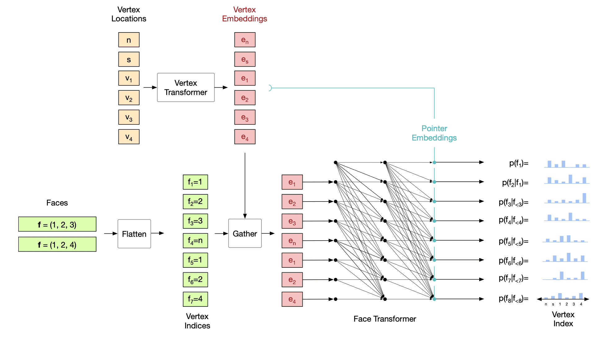
\[\begin{aligned} p(\mathcal{F}^{\text{seq}} \mid \mathcal{V} ; \theta) = \prod_{n=1}^{N_F} p (f_n \mid f_{< n}, \mathcal{V}; \theta) \end{aligned}\]and its distribution is also modeled by Transformer. Then the face model should address with variable length sequences of vertices. To deal with that issue, we generate pointer embeddings using an auto-aggressive network after each vertex embedding step as in mesh pointer networks.
First, for input vertices sequence of face model $\mathcal{V}$, obtain contextual embeddings \(\mathbf{e}_v\) of $\mathcal{V}$ using a Transformer encoder (vertices Transformer) $E$. Then, a gather (vector addressing) operation between \(\mathbf{e}^v\) and the flattened vertex indices that describe the faces is used to identify the embeddings associated with each vertex index. These gathered embeddings are processed with a masked Transformer decoder $D$ to output pointers $\mathbf{p}_k$ at each step. Finally, the target distribution can be obtained by comparing pointers with vertex embeddings with a dot-product:
\[\begin{aligned} \{ \mathbf{e}_v \}_{v = 1}^{N_v} & = E (\mathcal{V} ; \theta) \\ \mathbf{p}_k & = D(f_{< n}, \mathcal{V}; \theta) \\ p(f_n = k \mid f_{<n}, \mathcal{V}; \theta) & = \text{softmax}_k (\mathbf{p}_n^\top \mathbf{e}_k) \end{aligned}\]
Both vertices and faces model are trained to maximize the log-likelihood with respect to the model parameters $\theta$.
CAD Representation
Computer-aided design (CAD) among the numerous tools employed by engineers and designers. Its applications vary significantly, depending upon the user and the specific type of software in use. It’s not just having the the meshes, vertices, edges and faces but also more higher-level information such as geometric primitives and parametric curves and surfaces.
Here are some example works that address CAD representation.
-
Lambourne et al., BRepNet, CVPR 2021.
The authors of BRepNet demonstrate the superiority of applying convolutional kernels concerning oriented coedges. And this approach outperforms both network-based and heuristic methods in boundary representation (B-rep) segmentation tasks. The B-rep representation is a data structure comprised of faces, edges and vertices, glued together with topological connections between them. It is extensively employed for design and simulation, enabling to facilitate sophisticated operations in CAD modeling.
Feature vectors from a small collection of faces (grey), edges (black) and coedges (blue) adjacent to each coedge (red) are multiplied by the learnable parameters in the kernel. The hidden states arising from the convolution can then be pooled to perform face segmentation.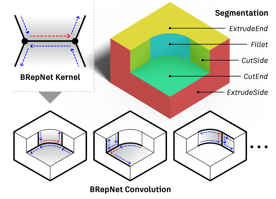
$\mathbf{Fig\ 27.}$ BRepNet convolutional kernels are defined based on coedges (dashed arrows).
(source: Lambourne et al., BRepNet, CVPR 2021.) -
Jayaraman et al., UV-Net, CVPR 2021.
B-rep data poses some distinctive challenges when utilized with neural networks, given the intricate nature of the data structure and its accommodation for diverse geometric and topological entities. UV-Net represents the geometry stored in the edges and faces of the B-rep by utilizing 1D and 2D UV-grids, which are structured sets of points uniformly sampled. Convolutional neural networks, both 1D and 2D, can be applied to these UV-grids to encode the edge and face geometry. And the topology is represented using a face-adjacency graph, where features from the face grids are stored as node features, and features from the edge grids are stored as edge features. A graph neural network is then employed to message-pass these features, obtaining embeddings for faces, edges, and the entire solid model.
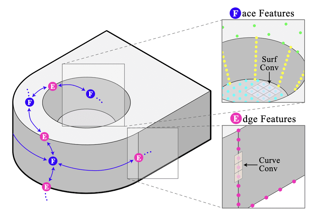
$\mathbf{Fig\ 28.}$ UV-Net builds features by sampling points on the edges and faces of solid models.
(source: Jayaraman et al., UV-Net, CVPR 2021.)
Summary
Although there are also many other types of 3D representations such as implicit representation. But these four are the most primitive representations for 3D data:
$\mathbf{Table\ 1.}$ Pros and Cons of 3D representations (source: Minhyuk Sung, KAIST)
Reference
[1] Maturana et al., VoxNet: A 3D Convolutional Neural Network for real-time object recognition, IROS 2015.
[2] Riegler et al., OctNet: Learning Deep 3D Representations at High Resolutions, CVPR 2017
[3] Wang et al., O-CNN: Octree-based Convolutional Neural Networks for 3D Shape Analysis, SIGGRAPH 2017
[4] Su et al., Multi-view Convolutional Neural Networks for 3D Shape Recognition, ICCV 2015
[5] Kalogerakis et al., 3D Shape Segmentation with Projective Convolutional Networks, CVPR 2017
[6] Václav Hlaváč, A mesh from a 3D point cloud
[7] Qi et al. “PointNet: Deep Learning on Point Sets for 3D Classification and Segmentation.” CVRP 2017.
[8] Florent POUX, Point Cloud Drawbacks, LinkedIn
[9] Stanford CS348a: Geometric Modeling and Processing
[10] Wikipedia, Polygon Mesh
[11] What is a Polygon Mesh and How to Edit It?
[12] Steve Marschner, Cornell CS4620 Fall 2014, Lecture 2
[13] Hanocka et al., MeshCNN: A Network with an Edge, SIGGRAPH 2019.
[14] CGAL, Triangulated Surface Mesh Simplification
[15] Yao et al., Quadratic Error Metric Mesh Simplification Algorithm Based on Discrete Curvature, 2015
[16] Nash et al., PolyGen: An Autoregressive Generative Model of 3D Meshes, ICML 2020.
[17] CSC2547 PolyGen: An Autoregressive Generative Model of 3D Meshes
[18] Lambourne et al., BRepNet: A topological message passing system for solid models, CVPR 2021.
[19] Wikipedia, Boundary representation
[20] Jayaraman et al., UV-Net: Learning from Boundary Representations, CVPR 2021.
Leave a comment