
[Graphics] Rendering Pipeline
Introduction
At the most basic level, the graphics pipeline, or rendering pipeline delineates a series of operations facilitating the transformation of a 3D object into a 2D pixel coordinate on the screen. It accommodates descriptions of 3D objects in terms of vertices of primitives (such as triangle, point, line and quad), and yields the color values for the pixels on the display. Broadly, the 3D graphics rendering pipeline consists of the following principal stages:
- Vertex Processing
The vertex shader processes and transforms individual vertices to map the 3D vertex locations to 2D screen positions. - Rasterization
The rasterizer converts the primitive (connected vertices), a continuous-geometry representation, into a set of fragments, the discrete geometry of the pixelized display, one by one. Therfore, a fragment is defined for a pixel location covered by the primitive on the screen and thus can be treated as a pixel in 3D spaces which is aligned with the pixel grid. Also, it possesses the attributes such as position, color, normal and texture to determine the rendering output of the pixel. Not programmable and specified by harware. Not programmble. - Fragment Processing
The fragment shader processes individual fragments and determines its color through various operations such as texturing and lighting. - Output Merging
The output merger combines the fragments of all primitives (in 3D space) into 2D color-pixel for the display. Not programmable.
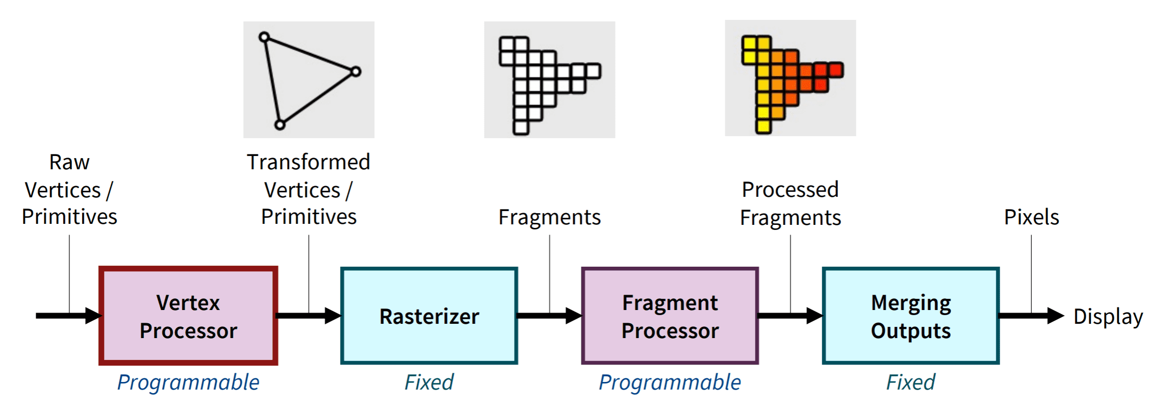
In modern GPUs, the vertex processing stage and fragment processing stage are programmable, known as vertex shader and fragment shader to operate the developer’s custom transformations for vertices and fragments. In contrast, the rasterizer and output merger are hard-wired stages that perform fixed but configurable functions. This is because there is no motivation for modifying the techniques for them and a special-purpose system allows for high efficiency. See [16].
Homogeneous Coordinates
Suppose we have the 2D point $(x, y)$ is given, and we’ve been exploring methods to represent translation
\[\begin{aligned} x^\prime & = x + x_t \\ y^\prime & = y + y_t \end{aligned}\]using a matrix $\mathbf{M} \in \mathbb{R}^{2 \times 2}$. However, it becomes evident that there’s simply no way to achieve this by multiplying $(x, y)$ by a $2\times2$ matrix alone. One approach to incorporate translation into our system of linear transformations is to assign a distinct translation vector to each transformation matrix. (In this setup, the matrix handles scaling and rotation, while the vector manages translation.) While this approach is feasible, the bookkeeping becomes cumbersome, and the rule for composing two transformations is not as straightforward and elegant as with linear transformations.
Instead, we introduce an extra dimension, augmenting $(x, y)$ by 3D vector $(x, y, 1)$ and use $3 \times 3$ matrices given by
\[\left[\begin{array}{ccc} m_{11} & m_{12} & x_t \\ m_{21} & m_{22} & y_t \\ 0 & 0 & 1 \end{array}\right]\]The above technique is called homogeneous coordinates, serving as a coordinate system for projective geometry, akin to Cartesian coordinates in Euclidean geometry. Homogeneous coordinates were first introduced by August Ferdinand Möbius in 1827. It has been discovered that the geometric manipulations employed in the graphics pipeline can be effectively carried out in a 4D coordinate space. Furthermore, this additional dimension offers more advantages than simply facilitating the representation of transformation matrices. As we will explore, it can also function as a means to retain depth information in perspective projection.
Homogeneous coordinates, therefore, are employed nearly universally to represent transformations in graphics systems including the graphics pipeline that is characterized by a sequence of matrix-vector multiplications. Specifically, homogeneous coordinates form the foundation of the design and operation of renderers implemented in graphics hardware. Hence we start by representing our 3D point $\mathbf{p}$ as a homogeneous vector with four elements:
\[\mathbf{p} = \left[\begin{array}{c} x \\ y \\ z \\ 1 \end{array}\right]\]For whom wonders the reason why it is called “homogeneous”, please refer to this post written by Songho Ahn.
Vertex Processing
In the process of rendering a 3D scene, objects must be projected onto a 2D screen through a simulated camera. Each object, along with the camera itself, possesses its unique position and orientation within the virtual world. Consequently, the surfaces of a model should undergo a series of transformations across various coordinate spaces before finally appearing as pixels on the screen. For these purposes, in the vertex processing stage, the vertex shader (A shader in the rendering pipeline is a synonym of a program) performs various transformations on every input vertex of objects and passes to the rasterizer. The vertex process is characterized by applying a series of transformations as shown:
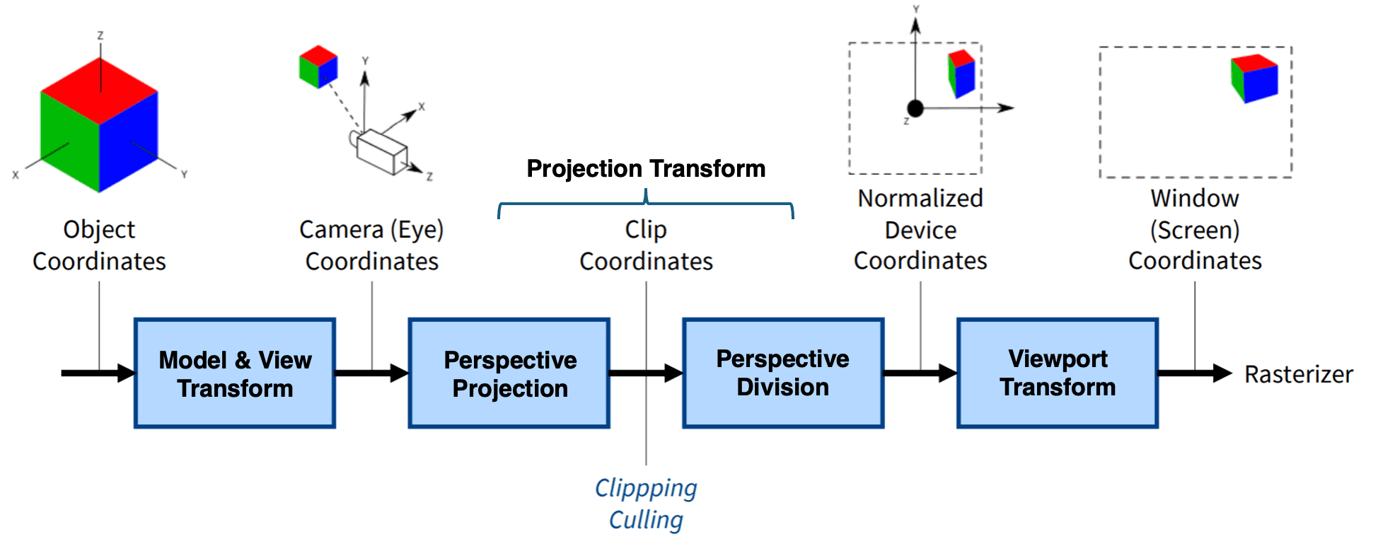
1. Model Transform
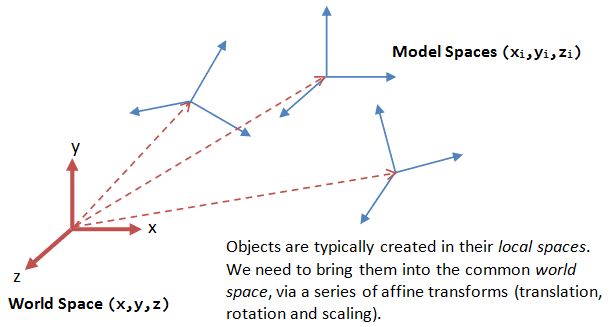
The vertex of 3D object is originally defined in its own coordinate system called object space. For example, if you load a 3D model from a file, each vertex of this model will be defined with respect to some local coordinate origin, which could be in the middle of the object. Say you are modeling a room with several identical chairs in it. You only need a single 3D model of a chair and then you create several copies of that and place them in the room. The 3D chair model will have its own origin and all points in the file will be defined with respect to that. This is object space.
To place each chair at a different position in the room, which now has another coordinate origin, e.g. the corner or center of the room, we need to transform the vertices from their local spaces to the world space, which is common to all the objects. This is known as the model transform, or world transform.
The model transform consists of the sequence of rotation, translation, and scale operations to transform the vertices of the 3D object from object space into world space. Mathematically, the transform can be expressed by multiplying the vertex with the $4 \times 4$ model matrix $\mathbf{M}$ as
\[\mathbf{p}_{\textrm{world}} = \mathbf{M} \mathbf{p}\]$\mathbf{M}$ is usually a combination of rotation, translation, and scale matrices, combined by multiplication. (Note that the order of these multiplications matters.) Below is the summary of these basic transformations.
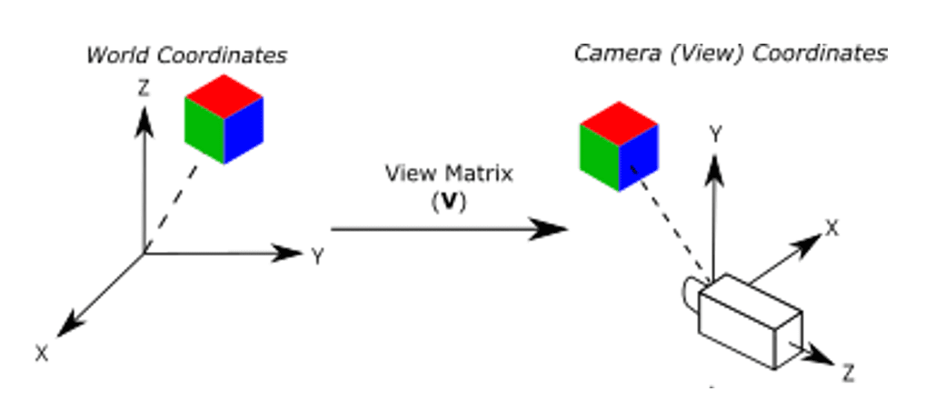
2. View Transform
After the model transform, all the objects are assembled into the world space. We shall now place the camera to capture the view. The view transform is described by another $4 \times 4$ matrix $\mathbf{V}$ called the view matrix, and transforms the point from world space to camera space (also called view space, or eye space).
\[\mathbf{p}_{\textrm{camera}} = \mathbf{V} \mathbf{p}_{\textrm{world}} = \mathbf{V} \mathbf{M} \mathbf{p}\]
We position the camera onto the world space by specifying three view parameters: eye, center and up, in world space.
-
eye $(e_x, e_y, e_z)$
3D point that defines the location of the camera.
-
center $(c_x, c_y, c_z)$
3D point that denotes the point in world coordinates that the camera is aiming at (e.g. at the center of the world or an object)
-
up $(u_x, u_y, u_z)$
3D vector that denotes the upward orientation of the camera roughly. It is typically coincided with the y-axis of the world space. Also, it is roughly orthogonal to center, but not necessary.
With these parameters, we can specify the basis $(\mathbf{x}_c, \mathbf{y}_c, \mathbf{z}_c)$ for the camera space. Conventionally, we set $z_c$ to be the opposite of $\textrm{center}$ $(c_x, c_y, c_z)$, i.e., $\textrm{center}$ is pointing at the $-z_c$. Then we obtain the direction of $x_c$ by taking the cross-product of $z_c$ and $\textrm{up}$ vector. Finally, we get the direction of $y_c$ by taking the cross-product of $x_c$ and $z_c$.
\[\mathbf{z}_c = \frac{\textrm{eye} − \textrm{center}}{\lVert \textrm{eye} − \textrm{center} \rVert}, \quad \mathbf{x}_c = \frac{\textrm{up} \times \mathbf{z}_c}{\lVert \textrm{up} \times \mathbf{z}_c \rVert}, \quad \mathbf{y}_c = \mathbf{z}_c \times \mathbf{x}_c\]Now, the world space is represented by standard orthonormal bases $(\mathbf{e}_1, \mathbf{e}_2, \mathbf{e}_3)$, where $\mathbf{e}_1=(1, 0, 0)$, $\mathbf{e}_2=(0, 1, 0)$ and $\mathbf{e}_3=(0, 0, 1)$, with origin at $\mathbf{0}=(0, 0, 0)$, and the camera space has orthonormal bases $(\mathbf{x}_c, \mathbf{y}_c, \mathbf{z}_c)$ with origin at $\textrm{eye}=(e_x, e_y, e_z)$. Hence the view matrix $\mathbf{V}$ consists of two operations: a translation for moving the entire world such that the camera is in the origin, followed by a rotation for rotating the world around the new origin. To obtain the view matrix, we have the following 4 constraints:
- The view matrix $\mathbf{V}$ should transform the vector $\mathbf{x}_c$ in the world space to be $(1, 0, 0)$ in the camera space.
- The view matrix $\mathbf{V}$ should transform the vector $\mathbf{y}_c$ in the world space to be $(0, 1, 0)$ in the camera space.
- The view matrix $\mathbf{V}$ should transform the vector $\mathbf{c}_c$ in the world space to be $(0, 0, 1)$ in the camera space.
- The camera should be standing at the origin in the camera space, i.e $\mathbf{V}$ should transform the center of the camera in the world space to be $(0, 0, 0)$ in the camera space.
Equivalently,
\[\mathbf{V} (\mathbf{T} \mathbf{R}) = \mathbf{I} \text{ where } \mathbf{T} = \begin{bmatrix} 1 & 0 & 0 & e_x \\0 & 1 & 0 & e_y \\0 & 0 & 1 & e_z \\0 & 0 & 0 & 1 \end{bmatrix}, \mathbf{R} = \begin{bmatrix} \mathbf{x}_c^x & \mathbf{y}_c^x & \mathbf{z}_c^x & 0 \\ \mathbf{x}_c^y & \mathbf{y}_c^y & \mathbf{z}_c^y & 0 \\ \mathbf{x}_c^z & \mathbf{y}_c^z & \mathbf{z}_c^z & 0 \\ 0 & 0 & 0 & 1 \end{bmatrix}\]Thus we have
\[\begin{aligned} \mathbf{V} & = \mathbf{R}^{-1} \mathbf{T}^{-1} = \mathbf{R}^\top \mathbf{T}^{-1} \\ & = \left[\begin{array}{cccc} \mathbf{x}_c^x & \mathbf{x}_c^y & \mathbf{x}_c^z & 0 \\ \mathbf{y}_c^x & \mathbf{y}_c^y & \mathbf{y}_c^z & 0 \\ \mathbf{z}_c^x & \mathbf{z}_c^y & \mathbf{z}_c^z & 0 \\ 0 & 0 & 0 & 1 \end{array}\right]\left[\begin{array}{cccc} 1 & 0 & 0 & -e_x \\ 0 & 1 & 0 & -e_y \\ 0 & 0 & 1 & -e_z \\ 0 & 0 & 0 & 1 \end{array}\right]=\left[\begin{array}{cccc} \mathbf{x}_c^x & \mathbf{x}_c^y & \mathbf{x}_c^z & -e_x \cdot \mathbf{x}_c \\ \mathbf{y}_c^x & \mathbf{y}_c^y & \mathbf{y}_c^z & -e_y \cdot \mathbf{y}_c \\ \mathbf{z}_c^x & \mathbf{z}_c^y & \mathbf{z}_c^z & -e_z \cdot \mathbf{z}_c \\ 0 & 0 & 0 & 1 \end{array}\right] \end{aligned}\]3. Projection Transform
Once the camera is positioned and oriented, our camera cannot hold all objects. Therefore, we need to decide what it can see (projection transform), and project the selected 3D objects onto the flat 2D screen (viewport transform).
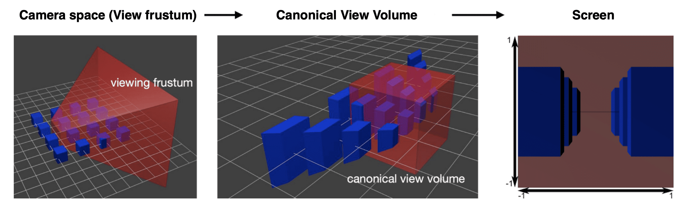
Projection transform is done by selecting a projection mode (perspective or orthographic) and converting the view volume (specifies field-of-view) into uniform cube called canonical view volume on normalized device coordinates (NDC) (standardized viewing volume representation). Objects sticking out from the view volume are clipped out of the scene (clipping). And objects totally outside the clipping volume are thrown away (view volume culling) and cannot be seen.
Projecting onto 3D unit cube instead of plane permits the preservation of depth information along $z$-axis. And this information will be utilized for depth test after vertex processing.
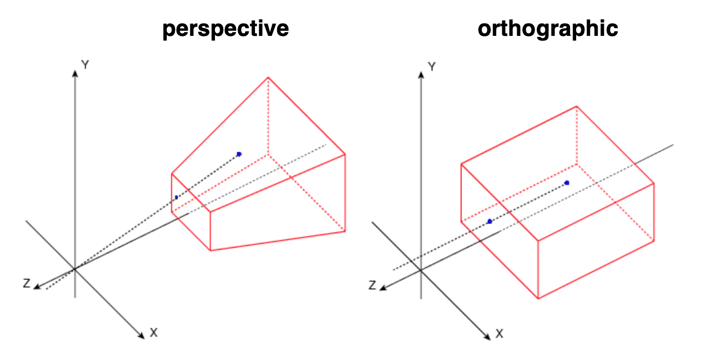
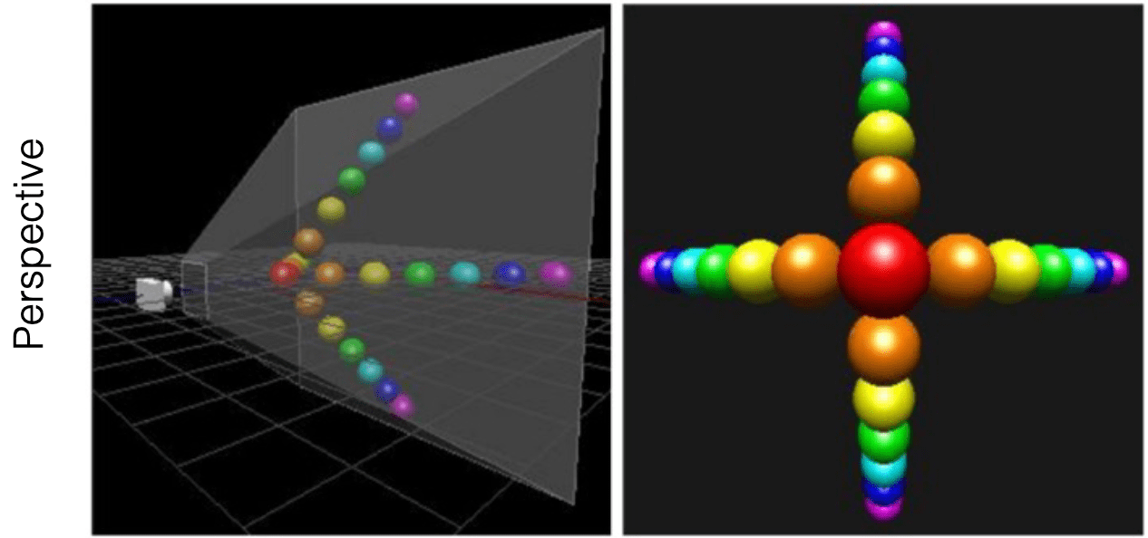
Perspective Projection
A perspective projection simulates a camera with a single center of projection, thereby encompassing effects such as perspective foreshortening and changes in relative object size with distance, commonly referred to as perspective effects. This model closely resembles the behavior of the human eye or a physical camera.
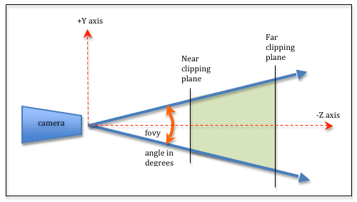
Hence, the view volume in perspective projection is represented by truncated pyramid, called view frustum, with $4$ parameters:
- fovy: the angle between the upper and lower sides of the viewing frustum
-
aspect: the aspect ratio of the viewing window, i.e.
width/height - near: the distance to the near plane along the $-z$ axis, i.e. camera lens
- far: the distance to the far plane along the $-z$ axis
Note that for a particular $z$, the height of the plane is calculated from the fovy, and then get the width from the aspect. Also, one should aware the sign of $z$-values. Marschner & Shirley define it as absolute $z$ coordinates, thus $\text{ near } > \text{ far }$ and both values are always negative. But OpenGL (and in this post) defines it as positive values, i.e. the distances of the near and far clipping plane from the camera. Thus $\text{ near } < \text{ far }$.
Then the perspective projection matrix \(\mathbf{P}_{\textrm{persp}}\) transforms the view frustum into a axis-aligned $2 \times 2 \times 2$ uniform volume:
\[\mathbf{p}_{\textrm{clip}} = \mathbf{P}_{\textrm{persp}} \cdot \mathbf{p}_{\textrm{camera}} = \mathbf{P}_{\textrm{persp}} \mathbf{V} \mathbf{M} \mathbf{p}\]$\color{#bf1100}{\mathbf{Proof.}}$
Step 1. Projection of $x$ and $y$ coordinate
Assume that we project an arbitrary vertex $\mathbf{v} = (x_c, y_c, z_c)$ in view frustum onto a plane of distance $d$ from the camera. And suppose that the plane is bounded by $- \textrm{aspect}$ to $\textrm{aspect}$ in $x$ coordinate and by $-1$ to $1$ in $y$ coordinate. Then, we can obtain $d = \tan^{-1} (\textrm{fovy} / 2)$ by vertical field of view, $\textrm{fovy}$.
Denote the projected point of vertex $\mathbf{x}$ by $\mathbf{v}_{\textrm{proj}} = (p_x, p_y, p_z)$. Then, by similarity we have
\[\frac{p_y}{d} = \frac{y_c}{z_c} \implies p_y = \frac{y_c\cdot d}{z_c} = \frac{y_c}{z_c \cdot \tan\left(\frac{\textrm{fovy}}{2}\right)} \\ \frac{p_x}{d} = \frac{x_c}{z_c} \implies p_x = \frac{x_c\cdot d}{z_c} = \frac{x_c}{z_c \cdot \tan\left(\frac{\textrm{fovy}}{2}\right)}\]To bound the projection ranges from $-\textrm{aspect}$ to $\textrm{aspect}$ in $x$ direction by $-1$ to $1$, finally we have
\[\begin{aligned} p_y & = \frac{y_c\cdot d}{z_c} = \frac{y_c}{z_c \cdot \tan\left(\frac{\textrm{fovy}}{2}\right)} \\ p_x & = \frac{x_c\cdot d}{z_c} = \frac{x_c}{z_c \cdot \textrm{ aspect } \cdot \tan\left(\frac{\textrm{fovy}}{2}\right)} \end{aligned}\]Step 2. Save $z$-depth in $w$ component
Note that both projected coordinates depend on $z_c$, inversely propotional to $z_c$. Also, the depth test after vertex processing still needs the $z$ value. Therefore we copy $z$ value to the $w$ component:
\[\left[ \begin{array}{cccc} \frac{1}{\textrm{aspect}\cdot\tan(\frac{\textrm{fovy}}{2})}&0&0\\ 0&\frac{1}{\tan(\frac{\textrm{fovy}}{2})}&0&0\\ 0&0&a&b\\ 0&0&1&0 \end{array} \right]\]And we will divide all clip coordinates by $w$ component in the last step. It is called perspective division.
Step 3. Projection of $z$ coordinate
Now we need to bound the $z$ range by $[−1,1]$ for all points between the near and far plane $[-\textrm{near}, -\textrm{far}]$ (Note that view frustum is along the $-z$-axis). Such a scaling and translation can be represented by linear transformation $f(z) = a \cdot z + b$. By considering perspective division and end points, we obtain the following equation system:
\[\begin{aligned} a - \frac{b}{\textrm{near}} & = -1 \\ a - \frac{b}{\textrm{far}} & = 1 \end{aligned}\]which leads to
\[a = - \frac{ \textrm{near } + \textrm{ far} }{\textrm{far } - \textrm{ near}} \\ b = - \frac{ 2 \times \textrm{near } \times \textrm{ far}}{\textrm{far } - \textrm{ near}}\]For derivation of asymmetric view frustum, see Song Ho Ahn’s blog post.
\[\tag*{$\blacksquare$}\]The space of view volume projected by perspective projection matrix commonly referred to as clip space. Recall that the projected view volume is not canonical since each coordinates are not divided by $z$ value in order to preserve the $z$-depth information. (See the derivation of perspective projection matrix.) Therefore, once all the vertices are transformed to clip space, a final operation called perspective division is performed where we divide the $x$, $y$ and $z$ components of the position vectors by the vector’s homogeneous $w$ component that saves the $z$ value. In the aftermath of perspective division, the clip space coordinates are now transformed into normalized device coordinates.
\[\mathbf{p}_{\textrm{clip}} = \begin{bmatrix} x_{\textrm{clip}} \\ y_{\textrm{clip}} \\ z_{\textrm{clip}} \\ w_{\textrm{clip}} \\ \end{bmatrix} \implies \mathbf{p}_{\textrm{NDC}} = \begin{bmatrix} x_{\textrm{clip}} / w_{\textrm{clip}} \in [-1, 1] \\ y_{\textrm{clip}} / w_{\textrm{clip}} \in [-1, 1] \\ z_{\textrm{clip}} / w_{\textrm{clip}} \in [-1, 1] \\ 1 \\ \end{bmatrix}\]Orthographic Projection
In contrast, an orthographic projection models a theoretical camera devoid of a center of projection. It simply flattens the world onto the film plane, where each pixel can be construed as a light ray that is parallel to all the other rays. This modeling is akin to the scenario where the camera is positioned at a significant distance from the world.
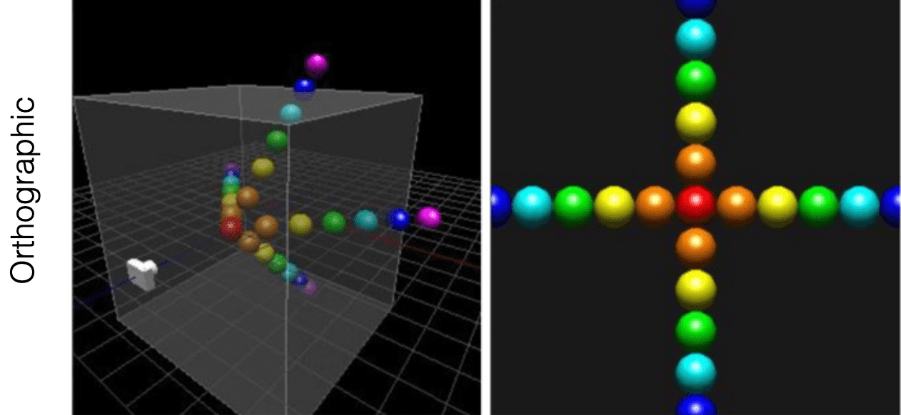
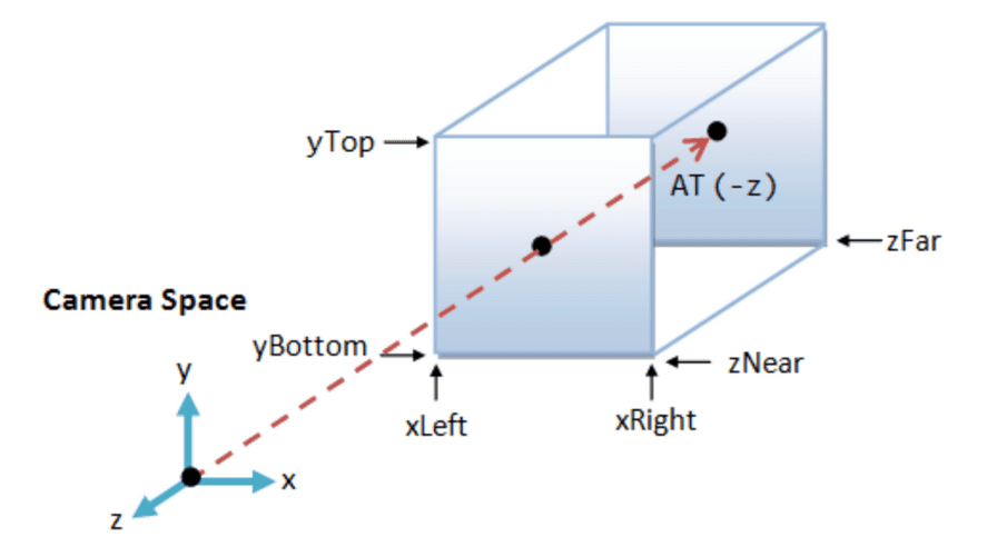
The view volume for orthographic projection is a parallelepiped instead of a frustum in perspective projection. And this is specified by the following $6$ parameters:
- left: Farthest left on the $x$-axis
- right: Farthest right on the $x$-axis
- bottom: Farthest down on the $y$-axis
- top: Farthest up on the $y$-axis
- near: the distance to the near plane along the $-z$ axis, i.e. camera lens
- far: the distance to the far plane along the $-z$ axis
Then the orthographic projection matrix $\mathbf{P}_{\textrm{ortho}}$ transforms the view volume into a axis-aligned $2 \times 2 \times 2$ uniform volume:
\[\mathbf{p}_{\textrm{NDC}} = \mathbf{P}_{\textrm{ortho}} \cdot \mathbf{p}_{\textrm{camera}} = \mathbf{P}_{\textrm{ortho}} \mathbf{V} \mathbf{M} \mathbf{p}\]$\color{#bf1100}{\mathbf{Proof.}}$
Note that all components in eye space can be linearly mapped to uniform volume. Therefore we just need to scale a rectangular volume to a cube, then translate it to the origin. For notation simplicity, we denote
\[\begin{aligned} \ell & = \textrm{left} \\ r & = \textrm{right} \\ t & = \textrm{top} \\ b & = \textrm{bottom} \\ f & = \textrm{far} \\ n & = \textrm{near} \\ \end{aligned}\]For $x$-coordinate, we have
\[p_x = \frac{1 - (-1)}{r - \ell} x_c + \beta\]and by substituting $(r, 1)$ for $(x_c, p_x)$, we obtain
\[\beta = - \frac{r + \ell}{r - \ell}\]Similarly, for $y$-coordinate, we have
\[p_y = \frac{1 - (-1)}{t - b} y_c + \beta\]and by substituting $(t, 1)$ for $(y_c, p_y)$, we obtain
\[\beta = - \frac{t + b}{t - b}\]Lastly, for $z$-coordinate, we have
\[p_y = \frac{1 - (-1)}{(- f) - (-n)} y_c + \beta\]and by substituting $(-f, 1)$ for $(z_c, p_z)$, we obtain
\[\beta = - \frac{f + n}{f - n}\]In summary, we obtain
\[\left[\begin{array}{cccc} \frac{2}{r-l} & 0 & 0 & -\frac{r+l}{r-l} \\ 0 & \frac{2}{t-b} & 0 & -\frac{t+b}{t-b} \\ 0 & 0 & \frac{-2}{f-n} & -\frac{f+n}{f-n} \\ 0 & 0 & 0 & 1 \end{array}\right]\] \[\tag*{$\blacksquare$}\]Therefore, an orthographic projection matrix directly maps coordinates to the 2D plane (screen) without requiring perspective division. However, in practice, such a projection yields unrealistic results because it disregards perspective. This limitation is addressed by the perspective projection matrix, which incorporates perspective effects into the projection.
4. Viewport Transform
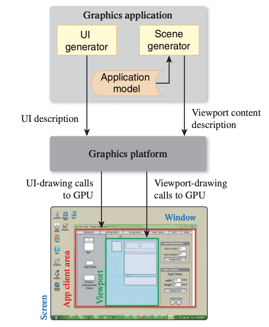
In a typical desktop/laptop setup, the application runs alongside a window manager responsible for allocating screen space to each application and managing window chrome (such as title bars, resize handles, close/minimize buttons, etc.). And the application primarily focuses on drawing within the client area, which constitutes the interior of the window, by utilizing calls to the graphics platform API that instructs the GPU to generate the desired rendering.
Usually, the application employs the client area for two main purposes: a portion of the area is dedicated to the application’s user interface (UI) controls, while the remaining space contains the viewport used to display the scene’s rendering. (It may or may not occupy the entire screen)
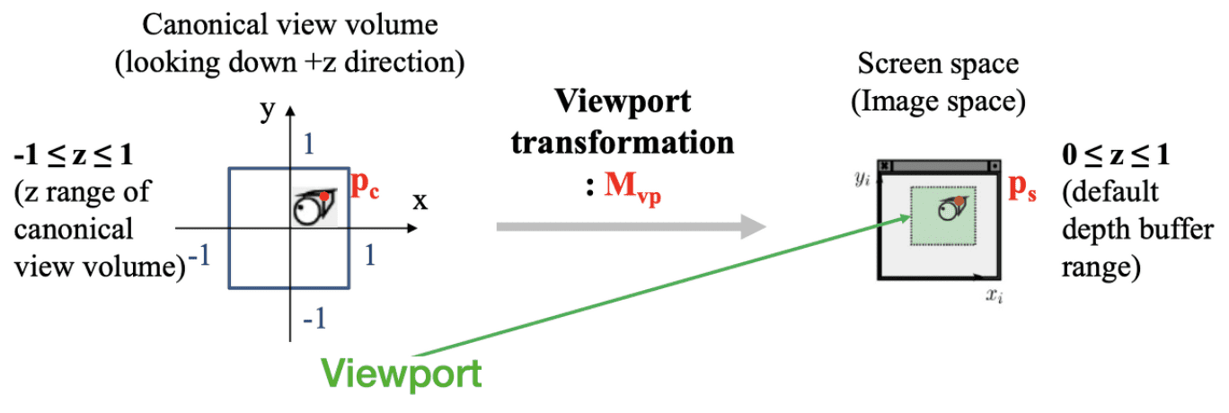
In other words, the viewport refers to a rectangular display area on the application window, measured in the screen coordinates (in pixels) with the origin typically located at the top-left corner. It determines both the size and shape of the display area, effectively mapping the projected scene captured by the camera onto the application window.
Therefore, the portion of the scene captured in the view volume from the projective transform is then projected to 2D screen, appearing in the viewport in the application’s window. Assuming that the viewport with $\textrm{width} \times \textrm{height}$ pixels and the top-left corner located at $(x, y)$ in the screen coordinates, we obtain
\[\mathbf{p}_{\textrm{NDC}} = \begin{bmatrix} x_{\textrm{NDC}} \in [-1, 1] \\ y_{\textrm{NDC}} \in [-1, 1] \\ z_{\textrm{NDC}} \in [-1, 1] \\ 1 \\ \end{bmatrix} \implies \mathbf{p}_{\textrm{screen}} = \begin{bmatrix} \frac{\textrm{width}}{2} (x_{\textrm{NDC}} + 1) + x \in [x, x + \textrm{width}] \\ \frac{\textrm{height}}{2} (y_{\textrm{NDC}} + 1) + y \in [y, y + \textrm{height}] \\ \frac{1}{2} (z_{\textrm{NDC}} + 1) \in [0, 1] \\ 1 \\ \end{bmatrix}\]where the transformation matrix $\mathbf{M}_{\mathrm{vp}}$ is given by
\[\mathbf{M}_{\mathrm{vp}}=\left[\begin{array}{cccc} \frac{\textrm { width }}{2} & 0 & 0 & \frac{\textrm { width }}{2}+x \\ 0 & \frac{\textrm { height }}{2} & 0 & \frac{\textrm { height }}{2}+y \\ 0 & 0 & \frac{1}{2} & \frac{1}{2} \\ 0 & 0 & 0 & 1 \end{array}\right]\]
The resulting coordinates are then sent to the rasterizer to turn them into fragments.
Rasterization
After the viewport transform, vertices of 3D object are now positioned on the viewport. To render a scene of 3D object as a next step, we must calculate the amount of light reaching each pixel of the image sensor within a virtual camera. Light energy is carried by photons, necessitating the simulation of photon physics within a scene. However, simulating every photon is impractical, so we must sample a subset of them and extrapolate from those samples to estimate the total incoming light. Therefore, rendering can be viewed as a process of sampling and the images are rendered by sampling the pixels along all viewing rays and calculating the optical properties.
One of the most dominant strategies for rendering, rasterization, converts vertex representation to pixel representation; determines the pixels that a given primitive (such as triangle, quad, point and line) covers on the screen, so that we can compute the colors of each covered pixel. The output of the rasterizer is a set of fragments. Fragment is the data aligned with the pixel-grid, containing its own set of attribute values such as position, color, normal, and texture. Therefore, for each pixel, corresponding fragment will determine the rendering of a pixel.
Rasterization serves as the cornerstone technique employed by GPUs to generate 3D graphics. Despite considerable advancements in hardware technology since the inception of GPUs, the fundamental methodologies they employ to render images have remained largely unaltered since the early 1980s. It is commonly compared to another methodology for rendering termed ray tracining, where it considers each pixel in turn and finds the objects that influence its color. (Rasterization instead considers each geometric object in turn.) The ray tracing will be covered in next posts.
1. Triangle Preprocessing
Given the transformed vertices for 3D object, the first thing to do is find the equation to form the primitives (triangle). Given 3 vertices
\[\mathbf{p}_j = \left[\begin{array}{c} x_j \\ y_j \\ z_j \\ 1 \\ \end{array}\right]\]where $j = 0, 1, 2$, edges of the triangle formed by 3 vertices are given by the edge equation:
\[\begin{aligned} E_{01} (x, y) & \equiv (y_1 - y_0) x + (x_0 - x_1)y + x_1 y_0 - x_0 y_1 = 0 \\ E_{12} (x, y) & \equiv (y_2 - y_1) x + (x_1 - x_2)y + x_2 y_1 - x_1 y_2 = 0 \\ E_{20} (x, y) & \equiv (y_0 - y_2) x + (x_2 - x_0)y + x_0 y_2 - x_2 y_0 = 0 \end{aligned}\]Each edge equation segments a planar region into three parts: a boundary, and two half-spaces. The boundary is identified by points where the edge equation is equal to zero. The half-spaces are distiguished by differences in the edge equation’s sign. We can choose which half-space gives a positive sign by multiplication by -1. Therefore, we scale all three edges so that their negative halfspaces are on the triangle’s exterior.
Why Triangles?
Triangles have many inherent benefits:
- Triangles are minimal
Triangles are determined by just 3 points or 3 edges; - Convex Polygons
An object is convex if and only if any line segment connecting two points on its boundary is contained entirely within the object or one of its boundaries.
Regardless of a triangle’s orientation on the screen, a given scan-line (the line that we loops the pixels in triangles for coverage determination; details in the next section) of triangle will contain only a single segment of that triangle. This significantly simplifies rasterization processes.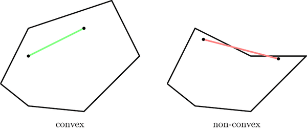
$\mathbf{Fig\ 14.}$ Convexity of polygons (source: INGInious) - Triangles Can Approximate Arbitrary Shapes
Any 2-dimensional shape (or 3D surface) can be approximated by a polygon using a locally linear (planar) approximation. To enhance the accuracy of the fit, we only need to increase the number of edges.
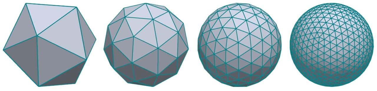
$\mathbf{Fig\ 15.}$ Polygonal approximation of sphere (source: Daniel Sieger) - Triangles Can Decompose Arbitrary Polygons
In case of a convex $n$-sided polygon, with ordered vertices $\{v_0, v_1, \cdots, v_n\}$ along the perimeter, can be trivially decomposed into triangles $\{(v_0,v_1,v_2), (v_0,v_2,v_3), (v_0,v_i,v_{i+1}), \cdots (v_0,v_{n-1},v_n)\}$. Moreover, a non-convex polygon can be also decomposed into triangles though it is non-trivial and somtimes have to introduce a new vertex.
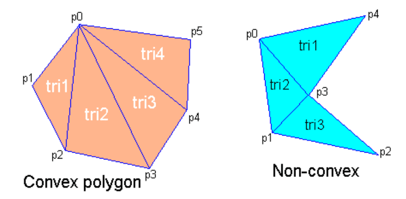
$\mathbf{Fig\ 16.}$ Decompositions of polygons (source: REFERENCE) - Hardware Efficiency
The modern GPUs are optimized for triangles due to their widespread use in 3D modeling. (This is somewhat a chicken and egg situation.)
2. Coverage Determination
After triangle primitives are drawn, for each primitive the associations of pixels in the image are determined. There are several possible methods to determine if a pixel overlaps a triangle and have its own pros and cons. One of the most generally utilized technique is Pineda’s method, proposed by Pineda et al. 1988. Recall that we defined the implicit functions called edge equations $E$ for primitives such that the value of points $P$ on the interior side of the primitive is positive:
\[E(P) = \begin{cases} > 0 & \quad \text{ if } P \text{ is on the interior} \\ = 0 & \quad \text{ if } P \text{ is on the boundary} \\ < 0 & \quad \text{ if } P \text{ is on the exterior} \end{cases}\]In this section, we will delve into this formulation more mathematically. Also recall that the form of edge equation:
\[\begin{aligned} E_{01} (x, y) & \equiv (y_1 - y_0) x + (x_0 - x_1)y + x_1 y_0 - x_0 y_1 \end{aligned}\]This is mathematically equivalent to the magnitude of the cross products between the vector \(\mathbf{p} - \mathbf{v}_0\) and \(\mathbf{v}_1 - \mathbf{v}_0\) where
\[\begin{aligned} \mathbf{p} & = (x, y, 1) \\ \mathbf{v}_0 & = (x_0, y_0, 1) \\ \mathbf{v}_1 & = (x_1, y_1, 1) \end{aligned}\]Formally,
\[\begin{aligned} E_{01} (x, y) & = \lVert (\mathbf{p} - \mathbf{v}_0) \times (\mathbf{v}_1 - \mathbf{v}_0) \rVert \\ & = \left\lVert {\begin{bmatrix}\mathbf {i} &\mathbf {j} &\mathbf {k} \\ x - x_0 & y - y_0 & 0 \\ x_1 - x_0 & y_1 - y_0 & 0 \\\end{bmatrix}} \right\rVert \\ & = \begin{vmatrix} x-x_0 & y-y_0 \\ x_1 - x_0 & y_1 - y_0 \end{vmatrix} \end{aligned}\]Therefore, we can determine whether the pixel belongs to a given primitive by just simply checking the sign of the edge function values, which is mathematically verified by cross product assuming right-hand rule convention. Note that $-z$-axis points into screen, conventionally. In view transform where the camera space is defined, we also set the direction that the camera views as $-z$-axis.
(Right) If the point is on the exterior of the triangle, at least one edge function will yield the negative value (source: current author)
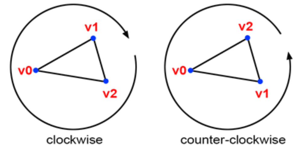
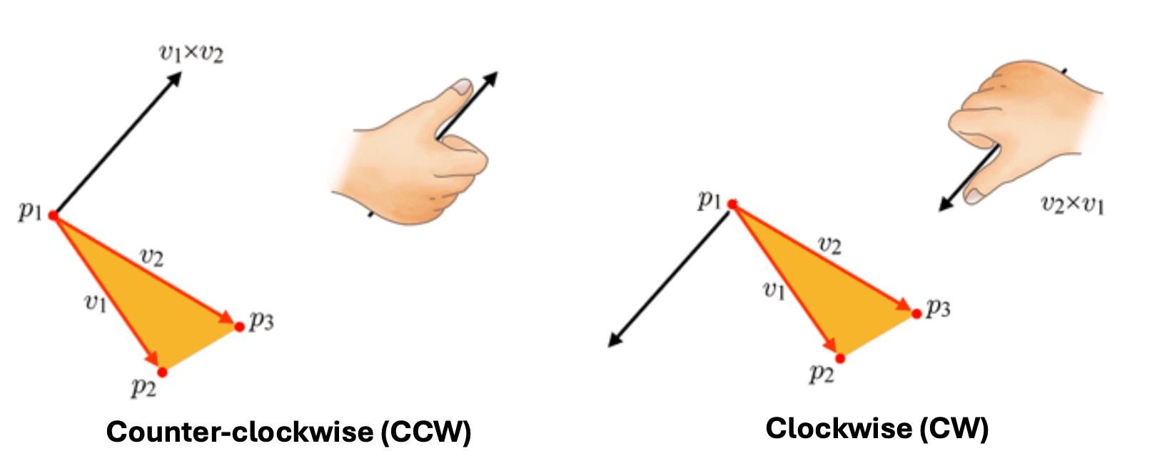
Notice that vertex ordering (winding order) matters: the ordering affects if points inside the triangle are positive or negative, as shown in $\mathbf{Fig\ 18}$. Generally, the common graphics APIs such as OpenGL and DirectX adopt the counter-clockwise order, but there is no universally mandated rule for selecting this order. Hence, depending on the winding order, one should adapt the edge functions by multiplication by $-1$ such that the interior gives a positive sign as mentioned in the previous section.
Fragment Processing
As the vertex shader yields the screen space vertices, the rasterizer, in turn, produces a collection of fragments within the screen space. These per-fragment data include a normal vector and the texture coordinates. Leveraging these data, the fragment shader determines the final color of each fragment, integrating two pivotal physical attributes:
- Lighting (often called shading)
- Texturing (often called texture mapping)
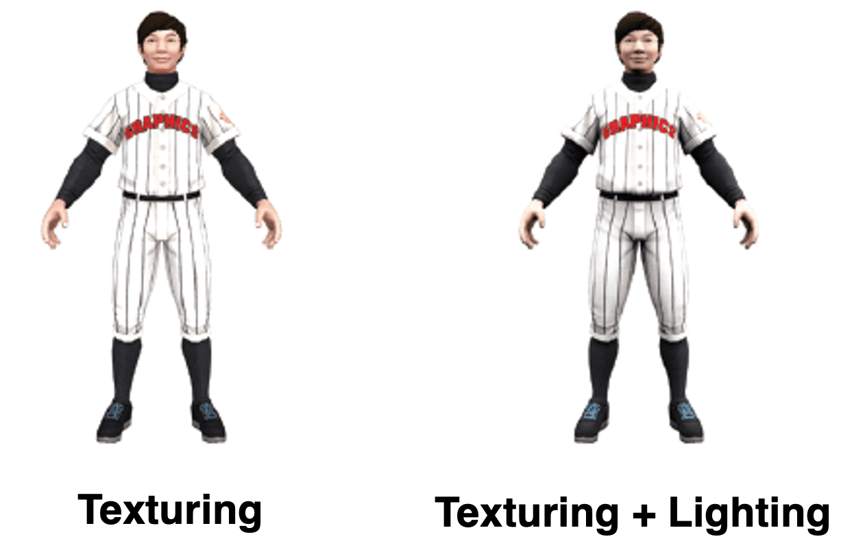
But due to their intricacies, these topics will be skipped and introduced in future posts in details.
Texture Mapping
Shading
Merging Outputs
Indeed, the fragment colors are not immediately displayed in the viewport. As the last step, the output merger merges all data (color and depth value of each pixel) of each primitive within our scene, obtained from the past processes that we have followed, to render them onto the display. It manages the frame buffer that consists of 3 kinds of buffers:
- Color buffer: memory space storing the pixels to be displayed.
- Depth buffer (Z-buffer): the same resolution as the color buffer and records the z-values of the pixels currently stored in the color buffer.
- Stencil buffer: extra data buffer, skipped in this post
As the low level, the frame buffer is just the designated memory to store the bitmapped image destined for the raster display device.Typically, it is stored on the graphic card’s memory, although integrated graphics such as Intel HD Graphics utilize the main memory for this purpose. And the frame buffer is characterized by its width, height, and depth. For instance, the frame buffer size for 4K UHD resolution with 32bit color depth would be $3840 \times 2160 \times 32$ bits.
1. Handling Visibility Problem
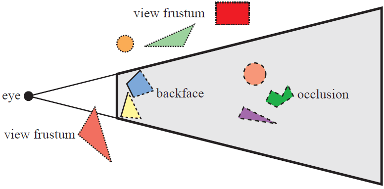
To render the scene captured by a camera, it’s crucial to identify which primitives and parts of primitives are not visible from our viewpoint. This consideration is known as visibility problem, which stands as one of the initial significant hurdles in rendering. There are several factors that render the primitives invisible:
- Primitives outside of the viewing frustum $\implies$ clipping & view volume culling
- Back-facing primitives $\implies$ back-face culling
- Primitives occluded by other objects closer to the camera $\implies$ occlusion culling (hidden-surface removal)
- Clipping & View Volume Culling
Indeed, clipping and view volume culling are typically performed during vertex processing, particularly in the projective transformation step. As vertices can be added to or removed from the triangle during this process, the clipping algorithms for polygons can be quite intricate. However, it’s worth noting that most graphics APIs, such as OpenGL, handle clipping by default. Therefore, we’ll skip delving into the details of these algorithms here. But if you’re interested, you can refer to the following resources for more information:
Recall that clipping and view volume culling are already mentioned and can be done in vertex processing, particularly in the projective transformation step. As vertices can be added to or removed from the triangle during this process, the clipping algorithms for polygons can be quite intricate. Moreover, most graphics APIs, such as OpenGL, handle clipping by default. Therefore, we’ll skip delving into the details of these algorithms here. But if you’re interested, you can refer to the following algorithms for more information:
-
Line clipping algorithms
- Cyrus–Beck
- Liang–Barsky
- Cohen–Sutherland
-
Polygon clipping algorithms
- Sutherland–Hodgman
- Weiler–Atherton
- Back-Face Culling
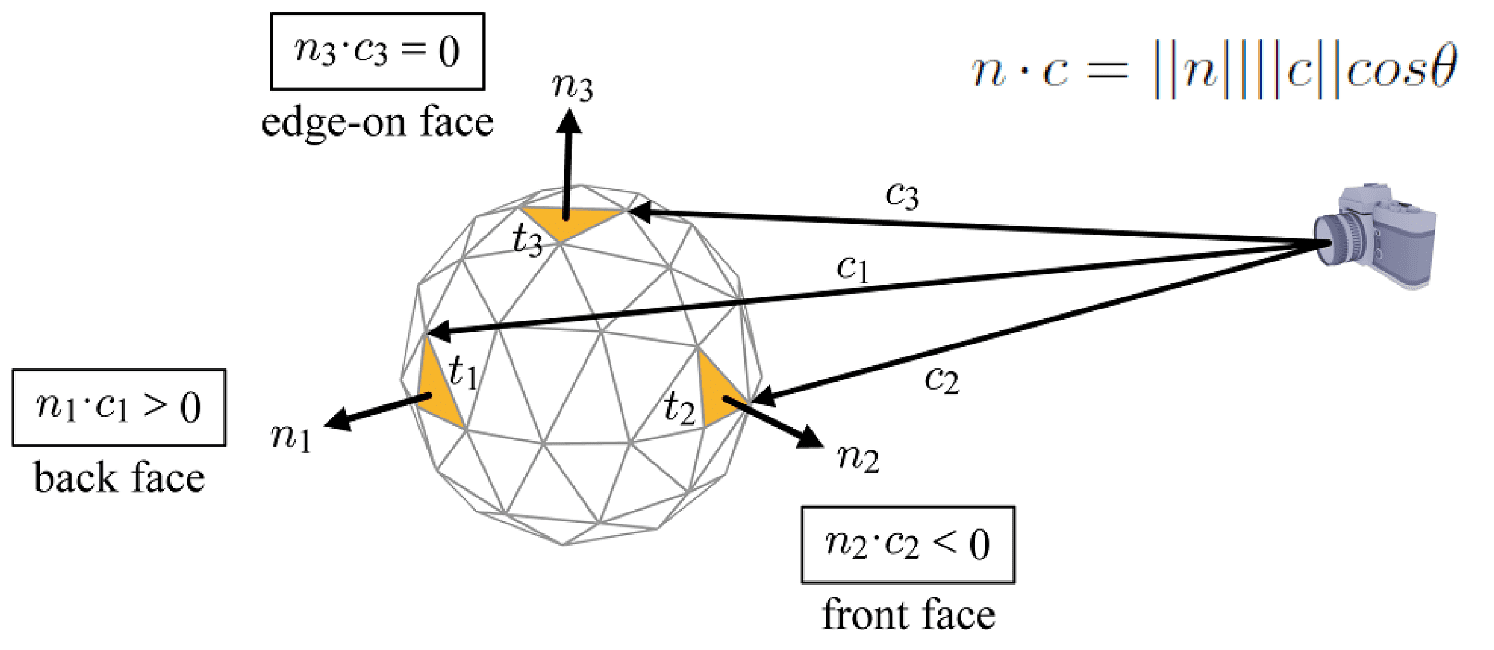
Polygons that face away from the camera (termed the back faces) are usually guaranteed to be overdrawn by polygons facing the camera (termed the front faces). Consequently, these back polygons can be culled, a process known as backface culling. One general approach to implement back-face culling is by utilizing the normal vector of primitives. Specifically, primitives are discarded if the dot product of their surface normal $\mathbf{n}$ and the camera-to-primitive \(\mathbf{c} = \mathbf{v}_0 - \mathbf{p}\) vector is non-negative:
\[(\mathbf{v}_0 - \mathbf{p}) \cdot \mathbf{n} \geq 0\]where $\mathbf{p}$ is the view point, $\mathbf{v}_0$ is the first vertex of the primitive and $\mathbf{n}$ is its surface normal, defined as
\[\mathbf{n} = (\mathbf{v}_1 - \mathbf{v}_0) \times (\mathbf{v}_2 - \mathbf{v}_0)\]
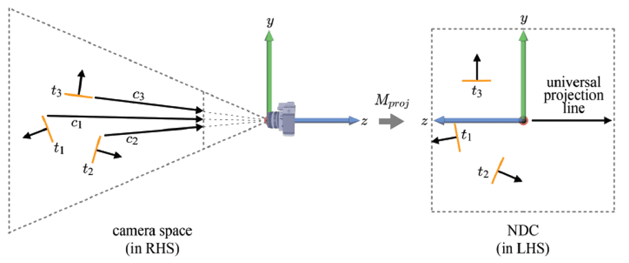
However, it’s essential to note that back faces should not always be culled. For instance, when rendering a hollow translucent sphere, the back faces must be visible through the front faces, necessitating that no faces are culled. Additionally, back-face culling is notably more efficient when conducted in the canonical view volume. This efficiency stems from the fact that in the canonical view volume, obtained via projection transform, the view point vector $\mathbf{p}$ is fixed along a universal projection line $(0, 0, 1)$.
Again, the winding order is crucial here because it essentially defines the orientation of its surface normal.
- Occlusion Culling
Occlusion culling, also referred to hidden-surface determination, hidden-surface removal, or visible-surface determination is the process of discarding of primitives that may be within the view volume but is obscured, or occluded, by other primitives closer to the camera. There are many techniques for occlusion culling:
In this section, we delve into two algorithms: painter’s algorithm that is the simplest algorithm, and depth testing that is the standard method for most graphics API.
Painter's algorithm
Painter’s Algorithm proceeds by sorting each primitives by depth and drawing from the farthest to the closest with overwriting. The term “painter’s algorithm” stems from the analogy to many painters where they begin by painting distant parts of a scene before parts that are nearer, thereby covering some areas of distant parts.

Despite its simplicity, there are three primary technical drawbacks that render the algorithm undesirable and time-consuming:
- Efficiency
Render each point on every primitives, even if that primitive is occluded in the output scene; Need to update the sorted graph whenever camera or object location is changed; - Cyclical Overlapping / Piercing Polygons
In some cases, the set of polygons is impossible to determine which polygon is above the others. The only solution to this is to divide these polygons into small pieces.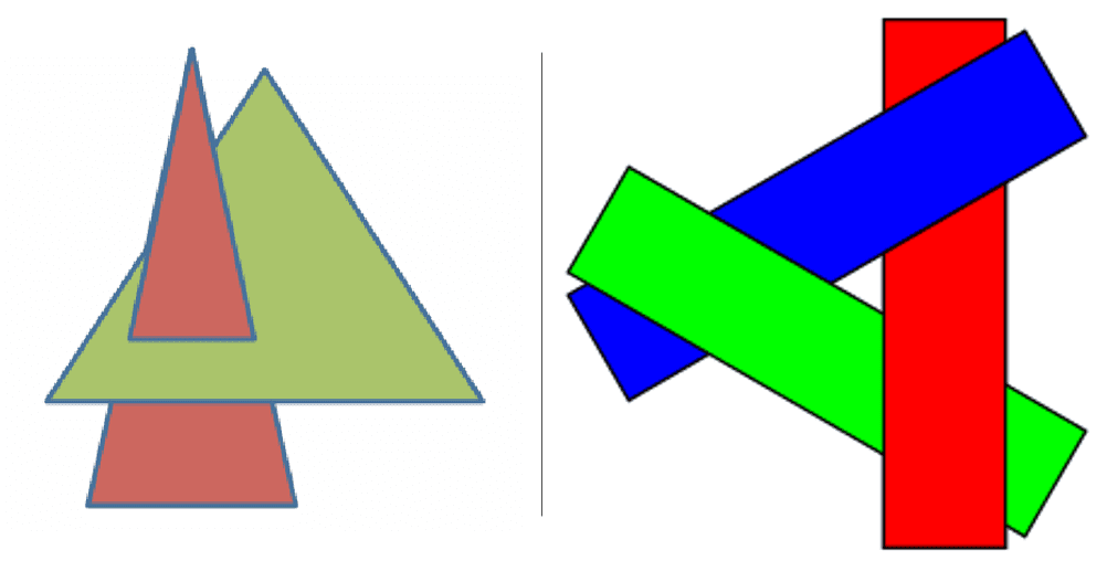
$\mathbf{Fig\ 25.}$ (Left) Piercing polygons (Right) Cyclical overlapping (wikipedia)
Depth Test (Z-buffering)
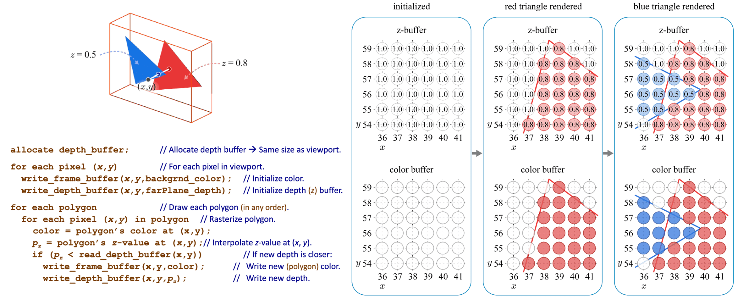
In most applications, to maintain the depth sort is daunting as it fluctuates whenever the view changes. One solution is to utilize the z-buffer (depth buffer), an ubiquitous and current standard technology in modern computing devices for 3D computer graphics such as computers, laptops, and mobile phones. Z-buffer is a 2D array that has the same dimension with the frame buffer (viewport), and only keeps track of the closest depth. With this buffer, we first initialize the per-pixel depth information in the z-buffer to max values, and then for each primitive overwrite the pixel information and update the depth when it is smaller than the current depth in the z-buffer.
Therefore, depth-buffer algorithm is possible to handle the challenging cases in painter’s algorithm, involving interpenetrating surfaces, since it operates at the pixel level (pixel-by-pixel) rather than the polygon level (polygon-by-polygon) basis of the painter’s algorithm. The next figure shows that the depth-buffer algorithm is robust to the piercing polygons:
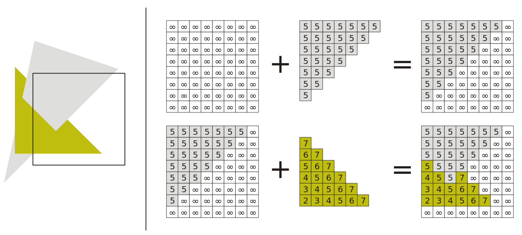
2. $\alpha$-blending
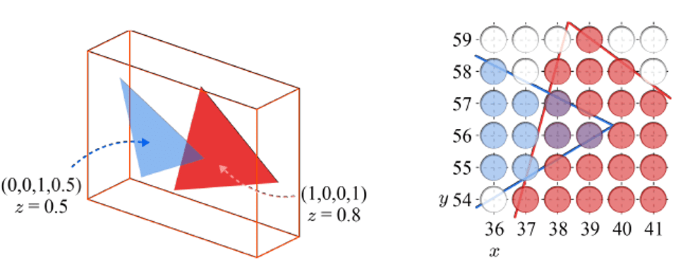
In the preceding section, we delved into the way how the processed fragment competes with the pixel stored in the color buffer, by replacing others or being occluded. However, this discourse remains pertinent only under the assumption of opaque front surfaces. Yet, in practical applications, not all the objects exhibit opaque; certain surfaces may be translucent (partially transparent). In computer vision/graphics, such degrees of opacity are generally specified by $\alpha$-value, conventionally normalized within the interval $[0, 1]$ where $0$ signifies totally transparent and $1$ signifies totally opaque. If the fragment is not completely opaque, then portions of its background object could show through. And the blending process, leveraging the alpha value of the fragment, is commonly referred to as $\alpha$-blending.

A typical blending equation is described as follows:
\[c = \alpha c_f + (1−\alpha) c_p\]where $c$ is the blended color, $\alpha$ represents the fragment’s opacity, $c_f$ is the fragment color, and $c_p$ is the pixel color stored in the current color buffer, i.e. backgroud color.
Although the depth testing generally allows the primitives to be processed in an arbitrary order, notice that for $\alpha$-blending, the primitives cannot be rendered in an arbitrary order and necessitates to be sorted. These primitives must be rendered subsequent to all opaque primitives, and in back-to-front sequence. Consequently, as the number of primitives increases, so does the computational overhead we incur.
Reference
[1] Huges et al. “Computer Graphics: Principles and Practice (3rd ed.)” (2013).
[2] MARSCHNER, S., AND SHIRLEY, P. 2016. Fundamentals of Computer Graphics. CRC Press.
[3] Stanford CS348A, Computer Graphics: Geometric Modeling/Processing
[4] Stanford EE267, Virtual Reality
[5] 3D Graphics with OpenGL Basic Theory
[6] KEA SIGMA DELTA, “Warp3D Nova: 3D At Last - Part 1”
[7] LEARN OpenGL, “Coordinate Systems”
[8] Rasterizing Triangles
[9] Stack Overflow, “Are triangles a gpu restriction or are there other rendering pathways?”
[10] ScratchPixel, Rasterization
[11] Pineda, Juan. “A parallel algorithm for polygon rasterization.” Proceedings of the 15th annual conference on Computer graphics and interactive techniques. 1988.
[12] Learn OpenGL, “Face culling”
[13] Han et al. Introduction to Computer Graphics with OpenGL ES. CRC Press, 2018.
[14] Wikipedia, Painter’s algorithm
[15] Wikipedia, Z-buffering
[16] Computer Graphics Stack Exchange, “Why do GPUs still have rasterizers?”
Leave a comment