
[Graphics] 3D Rotation via Quaternion
Introduction
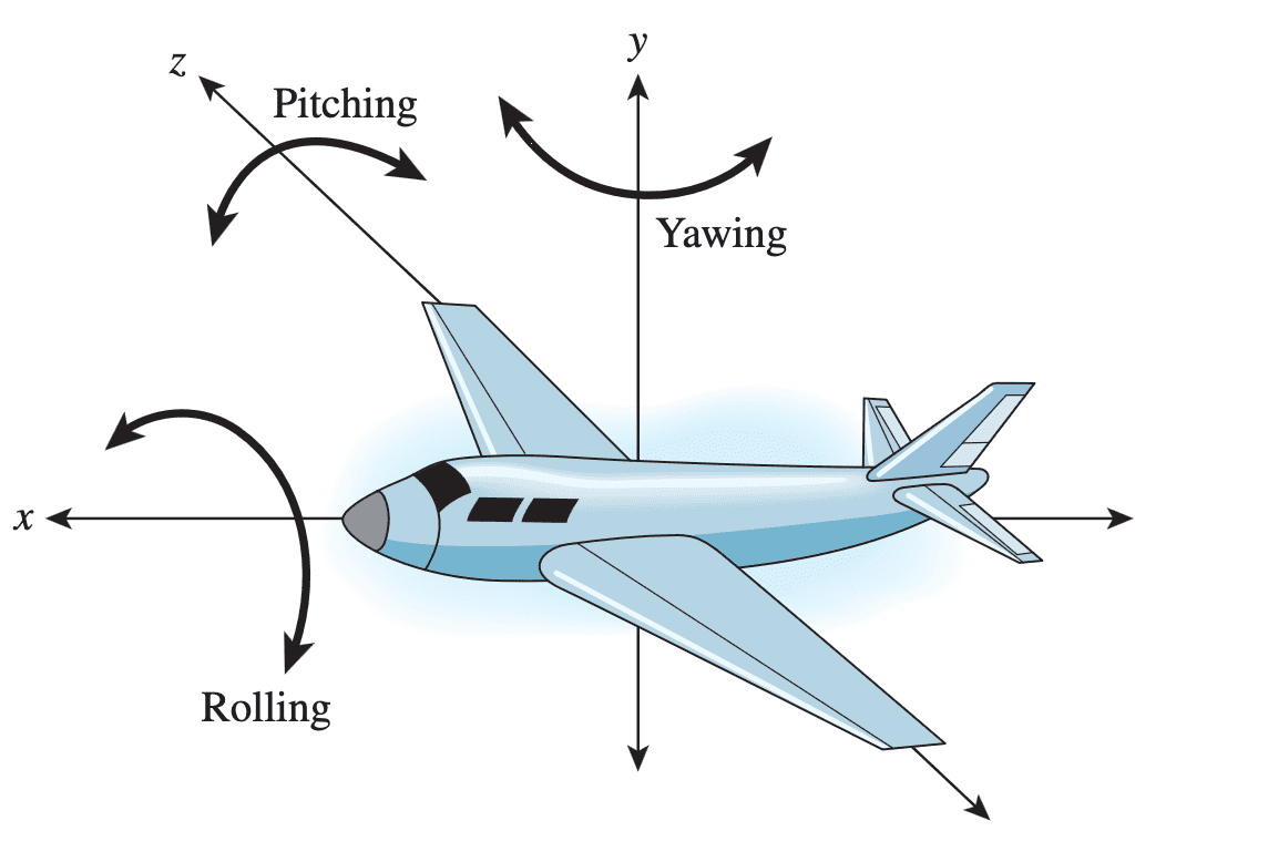
Mathematically representing orientation and rotation in three-dimensional space with is a complicated problem. Interpreting and performing computations with these representations is crucial in many systems that utilize a three-axis gyroscope. Euler angles representation is the most commonly used method for simulating a rotation through a sequence of 3 simpler rotations called roll, pitch, and yaw $(\psi, \phi, \theta)$, since it is the most intuitive and easily visualized system for representing orientation and rotation.
With the proper choice of roll, yaw, pitch $(\psi, \theta, \phi)$, the products of 3 rotation matrices represent all possible 3D rotations.
\[\begin{aligned} \mathbf{R} & =\left[\begin{array}{rrr} 1 & 0 & 0 \\ 0 & \cos \psi & -\sin \psi \\ 0 & \sin \psi & \cos \psi \end{array}\right]\left[\begin{array}{rrr} \cos \theta & 0 & \sin \theta \\ 0 & 1 & 0 \\ -\sin \theta & 0 & \cos \theta \end{array}\right]\left[\begin{array}{rrr} \cos \phi & -\sin \phi & 0 \\ \sin \phi & \cos \phi & 0 \\ 0 & 0 & 1 \end{array}\right] \\ & =\left[\begin{array}{rrr} \cos \theta \cos \phi & -\cos \theta \sin \phi & \sin \theta \\ \sin \theta \sin \psi \cos \phi + \cos \psi \sin \phi & - \sin \theta \sin \psi \sin \phi + \cos \psi \cos \phi & -\sin \psi \cos \theta \\ - \sin \theta \cos \psi \cos \phi + \sin \psi \sin \phi & \sin \theta \cos \psi \sin \phi + \sin \psi \cos \phi & \cos \psi \cos \theta \end{array}\right] \end{aligned}\]Problem: Gimbal Lock
However, to elucidate the values of $(\psi, \phi, \theta)$ that induce specific rotations is not intuitively obvious. For instance, $90^\circ$ rotation about the $x$-axis followed by $90^\circ$ rotation about the $y$-axis is equivalent to $120^\circ$ rotation about one of the major diagonals.
Moreover, although we have a one-to-one mapping from rotations to $(\psi, \phi, \theta)$, in certain special cases, such as when $\theta = \pi / 2$, multiple $(\psi, \phi)$ pairs pairs yield the same rotation matrix. Consequently, altering $\phi$ and $\psi$ simultaneously does not independently modify the object’s attitude, resulting in the loss of two degrees of freedom at once:
\[\begin{aligned} \mathbf{R}_{\theta = \frac{\pi}{2}} & = \left[\begin{array}{rrr} 0 & 0 & 1 \\ \sin \psi \cos \phi + \cos \psi \sin \phi & - \sin \psi \sin \phi + \cos \psi \cos \phi & 0 \\ - \cos \psi \cos \phi + \sin \psi \sin \phi & \cos \psi \sin \phi + \sin \psi \cos \phi & 0 \end{array}\right] \\ & = \left[\begin{array}{rrr} 0 & 0 & 1 \\ \sin (\psi + \phi) & \cos (\psi + \phi) & 0 \\ - \cos (\psi + \phi) & \sin (\psi + \phi) & 0 \end{array}\right] \\ \end{aligned}\]This phenomenon, known as gimbal lock, is a mathematical problem that occurs when Euler angles are used to represent rotations. And it is the reason why Euler angle representations are often considered mostly one-to-one, and why Euler angles are not regarded as an ideal method for characterizing rotations. It is termed gimbal lock because the pitch and roll axes of gimbal are “locked” together in this orientation. (Indeed, the Apollo 11 spacecraft famously had a gimbal lock problem and required specific operation to avoid this situation.) For visualization, refer to the following YouTube video.
One of the most popular solutions is to utilize quaternions. A quaternion is a complex number that represents a single orientation or rotation in three-dimensional space. While quaternions may initially appear more complex than Euler angles, it renders rotational computations simple to perform.
Quaternion
A quaternion $\mathbf{q}$ is a 4-dimensional complex number that takes the form $$ \mathbf{q} = a + b \mathbf{i} + c \mathbf{j} + d \mathbf{k} $$ where $a, b, c, d \in \mathbb{R}$ and $\mathbf{i}, \mathbf{j}, \mathbf{k}$ are unit imaginary numbers.
Quaternions are governed by a few special mathematical rules that differ from those surrounding conventional complex numbers. For example, quaternions are not communicative:
For two quaternions, $\mathbf{q}$ and $\mathbf{p}$, $\mathbf{qp} \neq \mathbf{pq}$. This stems from the fundamental formula for quaternion multiplication estabilished by Hamilton (the unit imaginary numbers are not communicative). Multiplication between the unit imaginary numbers follow the following rules: $$ \begin{array}{ll} \mathbf{i j}=\mathbf{k} & \mathbf{j i}=-\mathbf{k} \\ \mathbf{j k}=\mathbf{i} & \mathbf{k j}=-\mathbf{i} \\ \mathbf{k i}=\mathbf{j} & \mathbf{i k}=-\mathbf{j} \end{array} $$
The conjugate of a quaternion $\mathbf{q}$, notated as $\mathbf{q}^*$ or $\bar{\mathbf{q}}$, is defined as: $$ \mathbf{q}^* = a - b \mathbf{i} - c \mathbf{j} - d \mathbf{k} $$ where $\mathbf{q} = a + b \mathbf{i} + c \mathbf{j} + d \mathbf{k}$. The norm (magnitude) of a quaternion $\mathbf{q}$, notated as $\lvert \mathbf{q} \rvert$, is defined as: $$ \lvert \mathbf{q} \rvert = \sqrt{a^2 + b^2 + c^2 + d^2} = \sqrt{\mathbf{q} \mathbf{q}^*}. $$ The inverse, or reciprocal of $\mathbf{q}$ is given by $$ \mathbf{q}^{-1} = \frac{\mathbf{q}^*}{\lvert \mathbf{q} \rvert^2} $$
Now, to formulate the 3D rotation with quaternion, we define the following map from quaternions to quaternions:
The conjugation of $\mathbf{p}$ by $\mathbf{q}$, notated as $C_\mathbf{q} (\mathbf{p})$, is defined as $$ C_\mathbf{q} (\mathbf{p}) = \mathbf{q} \mathbf{p} \mathbf{q}^*. $$
Then, if $\mathbf{q}$ is unit quaternion, the conjugation mapping $C_\mathbf{q} (\mathbf{p})$ turns out to be 3D rotation of $\mathbf{p}$ with $\mathbf{q}$:
- $C_\mathbf{p} \circ C_\mathbf{q} = C_\mathbf{pq}$; indeed, $C_\mathbf{q}$ is a linear map from quaternions to quaternions with the corresponding matrix $M(\mathbf{q})$: $$ \begin{aligned} & M(\mathbf{q})=M(a + b \mathbf{i}+c \mathbf{j}+d \mathbf{k})= \\ & \quad\left(\begin{array}{cccc} a^2+b^2+c^2+d^2 & 0 & 0 & 0 \\ 0 & a^2+b^2-c^2-d^2 & 2 b c-2 a d & 2 b d+2 a c \\ 0 & 2 b c+2 a d & a^2-b^2+c^2-d^2 & 2 c d-2 a b \\ 0 & 2 b d-2 a c & 2 c d+2 a b & a^2-b^2-c^2+d^2 \end{array}\right) \end{aligned} $$
- The norm of every row/column of $M(\mathbf{q})$ is $\vert \mathbf{q} \rvert^2 = a^2 + b^2 + c^2 + d^2$.
- All rows are orthogonal each other. So are columns.
- $\textrm{det}(M(\mathbf{q})) = \vert \mathbf{q} \rvert^8 = (a^2 + b^2 + c^2 + d^2)^4$
An advantage of quaternions over the matrix representation of rotations with Euler angles is that they enable us to easily deduce the axis and angle of rotation from the quaternion components as the following theorem. The main idea of the proof is Rodrigues’ Rotation Formula, which we will discuss in the next section.
Given unit quaternion $\mathbf{q} = a + b \mathbf{i} + c \mathbf{j} + d \mathbf{k}$, it induces the 3D rotation with the angle $\theta$ along the axis $\vec{\mathbf{u}} \in \mathbb{R}^3$, where $ \vec{\mathbf{u}}$ and $\theta$ are given by the relations $$ \vec{\mathbf{u}} = (b, c, d) \\ \cos \frac{\theta}{2} = a, \quad \text{ equivalently } \quad \sin \frac{\theta}{2} = \sqrt{b^2 + c^2 + d^2} $$
Here are some few remarks:
-
There is a two-to-one mapping from unit quaternion to 3D rotations; for each 3D rotation matrix $R$, there exist two distinct corresponding unit quaternions, $\pm \mathbf{q}$ since $M (\mathbf{q}) = M(-\mathbf{q})$.
In algebra (specifically, Lie group theory), such a mapping is called double cover, a two-to-one surjective homomorphism $$ \Phi: \textrm{SU}(2) \to \textrm{SO}(3), \quad \textrm{ker}(\Phi) = \{ \pm 1 \} $$ where $\textrm{SU}(2)$ denotes a special unitary group defined by $$ \textrm{SU}(2) = \{ U \in \mathbb{C}^{2 \times 2} : U^* = U^{-1}, \textrm{det}(U) = 1 \} $$ For the mathematical proof, see [3]. -
Observe the analogy to Euler's formula in 2D coordinates:
-
2D rotation
- The multiplication of unit complex numbers is the same as combining the 2D rotations: $$ e^{i\varphi_1} e^{i \varphi_2} = e^{i (\varphi_1 + \varphi_2)} $$
- By Euler's formula $e^{i \varphi} = \cos \varphi + i \sin \varphi$, for unit complex number $z = a + ib$ we have $$ \cos \varphi = a, \quad \text{ equivalently } \quad \sin \varphi = b $$
-
3D rotation
- The multiplication of unit quaternions is the same as combining the 3D rotations: $$ M(\mathbf{p}\mathbf{q}) = M(\mathbf{p})M(\mathbf{q}) $$
- By Rodrigues’ rotation formula, for unit quaternion $\mathbf{q}=a + b\mathbf{i}+c\mathbf{j}+d\mathbf{k}$ the rotation angle $\varphi$ and axis $\vec{\mathbf{u}}$ are given by the relations $$ \vec{\mathbf{u}} = (b, c, d) \\ \cos \frac{\varphi}{2} = a, \quad \text{ equivalently } \quad \sin \frac{\varphi}{2} = \sqrt{b^2 + c^2 + d^2} $$
-
2D rotation
Rodrigues’ Rotation Formula
To derive the formula, we first introduce the axis-angle representations for the rotation. One method of rotating in 3D space is to select a specific axis and rotate around that direction by a certain amount. Consider the rotation about an axis (unit vector) $\mathbf{k}$ with an angle $\theta$. For any given 3D vector $\mathbf{v} \in \mathbb{R}^3$, we decompose this vector into two components: \(\mathbf{v}_{\parallel}\) that is parallel to $\mathbf{k}$ and \(\mathbf{v}_{\perp}\) that is perpendicular to it:
\[\mathbf{v} = \mathbf{v}_{\parallel} + \mathbf{v}_{\perp} \\ \begin{aligned} \text{ where } & \mathbf{v}_{\parallel} = (\mathbf{v} \cdot \mathbf{k}) \mathbf{k} = (\mathbf{k} \mathbf{k}^\top) \mathbf{v} \\ & \mathbf{v}_{\perp} = \mathbf{v} - \mathbf{v}_{\parallel} \end{aligned}\]
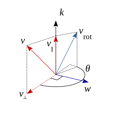
A rotation about $\mathbf{k}$ will not influence \(\mathbf{v}_{\parallel}\), but it will affect \(\mathbf{v}_{\perp}\). Specifically, this will introduce a new component $\mathbf{w} = \mathbf{k} \times \mathbf{v}$ that is perpendicular to both \(\mathbf{v}_{\perp}\) and the axis $\mathbf{k}$. Note that $\mathbf{k} \times \mathbf{v}$ can be expressed as a matrix multiplication involving a special matrix $\mathbf{K}$, i.e. $\mathbf{k} \times \mathbf{v} = \mathbf{K} \mathbf{v}$ where
\[\mathbf {K} =\left[{\begin{array}{rrr}0\ \,&-k_{z}&k_{y}\\k_{z}&0\ \,&-k_{x}\\-k_{y}&k_{x}&0\ \,\end{array}}\right] = -(\mathbf{I}_{3 \times 3} - \mathbf{k}\mathbf{k}^\top)\]Then the rotated point \(\mathbf{v}_{\textrm{rot}}\) will have the equation:
\[\begin{aligned} \mathbf{v}_{\textrm{rot}} & = \mathbf{v}_{\parallel} + \mathbf{v}_{\perp} \cos \theta + \mathbf{w} \sin \theta \\ & = (\cos \theta \cdot \mathbf{I}_{3 \times 3} + (1 - \cos \theta)(\mathbf{k}\mathbf{k}^\top) + \sin \theta \mathbf{K}) \mathbf{v} \\ & \equiv R(\mathbf{k}, \theta) \mathbf{v} \end{aligned}\]where $R(\mathbf{k}, \theta) = \mathbf{I}_{3 \times 3} + \mathbf{K} \sin \theta + \mathbf{K}^2 (1 - \cos \theta)$:
\[R(\mathbf{k}, \theta)=\left[\begin{array}{ccc} \cos \theta+k_x^2(1-\cos \theta) & k_x k_y(1-\cos \theta)-k_z \sin \theta & k_x k_z(1-\cos \theta)+k_y \sin \theta \\ k_y k_x(1-\cos \theta)+k_z \sin \theta & \cos \theta+k_y^2(1-\cos \theta) & k_y k_z(1-\cos \theta)-k_x \sin \theta \\ k_z k_x(1-\cos \theta)-k_y \sin \theta & k_z k_y(1-\cos \theta)+k_x \sin \theta & \cos \theta+k_z^2(1-\cos \theta) \end{array}\right]\]And this equation is termed Rodrigues’ Rotation Formula, an efficient algorithm for rotating a vector in space, given an axis and angle of rotation.
For given the unit vector $\mathbf{k}$ and an angle $\theta$, the rotation matrix $R(\mathbf{k}, \theta)$ about the axis $\mathbf{k}$ with the angle $\theta$ is given by $$ \begin{aligned} R(\mathbf{k}, \theta) & = \mathbf{I}_{3 \times 3} + \mathbf{K} \sin \theta + \mathbf{K}^2 (1 - \cos \theta) \\ & = \left[\begin{array}{ccc} \cos \theta+k_x^2(1-\cos \theta) & k_x k_y(1-\cos \theta)-k_z \sin \theta & k_x k_z(1-\cos \theta)+k_y \sin \theta \\ k_y k_x(1-\cos \theta)+k_z \sin \theta & \cos \theta+k_y^2(1-\cos \theta) & k_y k_z(1-\cos \theta)-k_x \sin \theta \\ k_z k_x(1-\cos \theta)-k_y \sin \theta & k_z k_y(1-\cos \theta)+k_x \sin \theta & \cos \theta+k_z^2(1-\cos \theta) \end{array}\right] \end{aligned} $$ where $\mathbf {K} =\left[{\begin{array}{rrr}0\ \,&-k_{z}&k_{y}\\k_{z}&0\ \,&-k_{x}\\-k_{y}&k_{x}&0\ \,\end{array}}\right] = -(\mathbf{I}_{3 \times 3} - \mathbf{k}\mathbf{k}^\top)$.
Note that $$ \begin{aligned} \textrm{trace}(\mathbf{R}) & = \textrm{trace}(\mathbf{I}) + (1 - \cos \theta) \textrm{trace}(\mathbf{k}\mathbf{k}^\top - \mathbf{I}) \\ & = 1 + 2 \cos \theta \end{aligned} $$ This provides us with a method to also recover the angle from the rotation matrix.
By comparing $R (\mathbf{k}, \theta)$ and $M(\mathbf{q})$ of unit quaternion $\mathbf{q} = a + b\mathbf{i} + c \mathbf{j} + d \mathbf{k}$, i.e. from the equation
\[R(\mathbf{k}, \theta) = \left[\begin{array}{ccc} a^2+b^2-c^2-d^2 & 2 b c-2 a d & 2 b d+2 a c \\ 2 b c+2 a d & a^2-b^2+c^2-d^2 & 2 c d-2 a b \\ 2 b d-2 a c & 2 c d+2 a b & a^2-b^2-c^2+d^2 \end{array}\right]\]we obtain the axis and angle of the rotation induced by $\mathbf{q}$. Firstly, from the sum of the diagonal,
\[\begin{aligned} & 3 a^2-b^2-c^2-d^2=4 a^2-1=3 \cos \theta+\left(k_x^2+k_y^2+k_z^2\right)(1-\cos \theta)=2 \cos \theta+1 \\ & \therefore a= \pm \sqrt{\frac{\cos \theta+1}{2}}=\cos \frac{\theta}{2} \end{aligned}\]By adding 2nd & 3rd diagonal entires,
\[\begin{aligned} & \left(a^2-b^2+c^2-d^2\right)+\left(a^2-b^2-c^2+d^2\right)=2 a^2-2 b^2=(\cos \theta+1)-2 b^2 \\ & \left(\cos \theta+k_y^2(1-\cos \theta)\right)+\left(\cos \theta+k_z^2(1-\cos \theta)\right)=2 \cos \theta+\left(1-k_x^2\right)(1-\cos \theta) \\ & \therefore b= \pm \sqrt{k_x^2\left(\frac{\cos \theta-1}{2}\right)}=k_x \sin \frac{\theta}{2} \end{aligned}\]Similarly, $c = k_y \sin \frac{\theta}{2}$ and $d = k_z \sin \frac{\theta}{2}$.
Here are some examples of 3D rotation with quaternions:
- Apply $90^\circ$ rotation along $y$-axis and subsequently $90^\circ$ rotation along $x$-axis is equivalent to $120^\circ$ rotation along the diagonal.
- Given a unit quaternion $\mathbf{q} = a + b \mathbf{i} + c\mathbf{j} + d \mathbf{k}$ with its corresponding rotation $R$, rotation matrix $R^{-1} = R^\top$ represent the rotation of conjugate of $\mathbf{q}$, $\mathbf{q}^*$ or equivalently $\mathbf{q}^{-1}$.
- Given two rotations represented with two unit quaternions $\mathbf{q}_0$ and $\mathbf{q}_1$, the unit quaternion for the relative rotation from $\mathbf{q}_0$ to $\mathbf{q}_1$ is given by $\mathbf{q}_1 \mathbf{q}_0^{-1}$.
$\mathbf{Proof.}$
(1)
\[\left( \frac{1}{2} + \frac{1}{2} \mathbf{i} \right) \left( \frac{1}{2} + \frac{1}{2} \mathbf{j} \right) = \frac{1}{2} + \frac{1}{2} \mathbf{i} + \frac{1}{2} \mathbf{j} + \frac{1}{2} \mathbf{k}\]Then $\vec{u} = (\frac{1}{2}, \frac{1}{2}, \frac{1}{2})$ and $\theta = 120^\circ$.
(2) It is trivial.
(3) Suppose the rotation with $\mathbf{q}_0$ rotates the object from the state $\mathcal{S}_0$ to the state $\mathcal{S}_1$, and the rotation with $\mathbf{q}_1$ rotates the object from the state $\mathcal{S}_0$ to the state $\mathcal{S}_2$. Then we’re interested in the rotation $M(\mathbf{r})$ such that rotates the object from $\mathcal{S}_1$ to $\mathcal{S}_2$. That is,
\[M(\mathbf{q}_1) = M(\mathbf{r}) M(\mathbf{q}_0)\]Thus,
\[M(\mathbf{r}) = M(\mathbf{q}_1) M^{-1}(\mathbf{q}_0) = M(\mathbf{q}_1) M(\mathbf{q}_0^{-1})\]and we obtain $\mathbf{r} = \mathbf{q}_1 \mathbf{q}_0^{-1}$.
\[\tag*{$\blacksquare$}\]Reference
[1] Huges et al. “Computer Graphics: Principles and Practice (3rd ed.)” (2013).
[2] Stanford CS348A, Computer Graphics: Geometric Modeling/Processing
[3] Supplementary Notes: “Spin, topology, SU(2)→SO(3) etc.” of University of Cambridge
[4] Wikipedia, Rodrigues’ rotation formula
[5] Chirgwin, B.H., and C. Plumpton. A Course of Mathematics for Engineers and Scientists. vol. 6. Oxford: Pergamon, 1966. pp. 4–17.
[6] Erik B. Dam & M. Koch & M. Lillholm, “Quaternions, Interpolation and Animation”, Technical Report DIKU-TR-98/5, 1998, Department of Computer Science, University of Copenhagen
[7] Geometric Tools Engine, Documentation
[8] Ken Shoemake, “Animating Rotation with Quaternion Curves”, International Conference on Computer Graphics and Interactive Techniques, Volume 19, Number 3, 1985
Leave a comment