
[Graphics] Radiometry & Photometry
In ray tracing, various physical phenomena related to the light such as reflection are taken account to rendering of scene. To precisely delineate how light is represented and simulated to compute images, we must first establish some background in radiometry—the study of the propagation of electromagnetic radiation in an environment.
Light
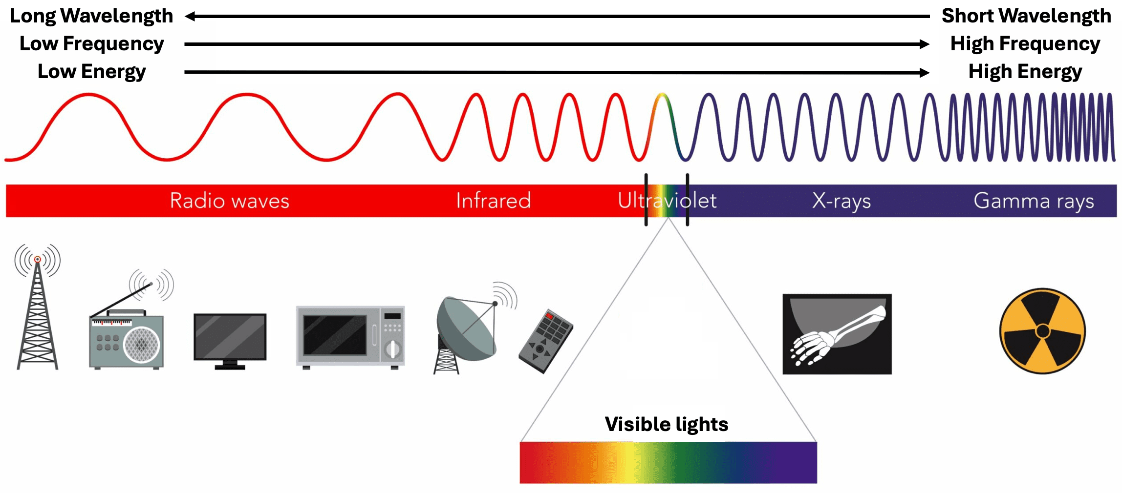
In theory, light is defined as the electromagnetic radiation, described in terms of a wave-like stream of mass-less particles called photons. Electromagnetic radiation transports energy through space, where each photon carries a small amount of energy called radiant energy. Therefore, the different types of radiation are characterized by the the amount of energy contained in the photons:
In general, a comprehensive and precise description of electromagnetic radiation and its behavior necessitates a profound knowledge of quantum electrodynamics and Maxwell’s electromagnetic field equations. Moreover, the perception of our eyes also requires the deep understanding of the physiology and psychology of the human visual system. Fortunately in computer graphics, our objectives are decidedly modest-we simply want to quantify what we observe and perceive. In general, we make the fundamental assumptions regarding the description of light in graphics and ignore the intricate physical properties associated with lights, such as polarization, interference, diffraction, and so forth.
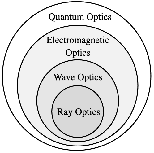
Computer graphics typically relies on the simplest of these models, known as ray optics or geometric optics. This model operates under several simplifications regarding the behavior of light. Fundamentally, within this model, light can only be emitted, reflected, and transmitted. Conversely, the complex effects described by the higher-level optics, such as diffraction and interference (wave optics), polarization and dispersion (electromagnetic optics), and fluorescence and phosphorescence (quantum optics) are completely ignored. Specifically:
-
Linearity
- The combined effect of light from various sources always equals the sum of the effects of each light individually
- This assumption proves useful in various situations, such as in the discussion of BRDF in this post.
- Nonlinear scattering behavior is typically observed only in physical experiments involving extremely high energies, making this assumption generally reasonable.
-
Photons travel in straight lines
- Represented by rays
- Wavelength « size of objects
- No diffraction, interference
-
No polarization
- Curiously, the polarization state of light is essentially imperceptible to humans without additional aids like specialized cameras or polarizing sunglasses.
-
Energy conservation
- When light scatters from a surface or from participating media, the scattering events can never produce more energy than they started with.
-
Steady state
- Rate of energy consumption is constant, thus flux (power) and energy are often interchangeable. This happens nearly instantaneously with light in realistic scenes, so it is not a limitation in practice. Note that phosphorescence also violates the steady-state assumption.
Although these assumptions may simplify the representation of light too much, we are still able to correctly simulate a wide range of physical phenomena. Moreover, it is indeed possible to include these complex effects if necessary. As examples, see Oh 2010 and Cuypers et al. 2012 that model the wave effects with Wigner distribution function.
Radiometry & Photometry
Radiometry is the detection and measurement of lights in any portion of the electromagnetic spectrum. (In practice, the term is usually limited to the measurement of ultraviolet (UV), visible (VIS), and infrared (IR) radiation using optical instruments.) It provides a set of techniques to describe light propagation and reflection and forms the basis of the derivation of a plethora of rendering algorithms.
On the other hand, photometry is the detection and measurement in terms of its perception by the human visual system, especially its brightness, of lights within the visible portion of the electromagnetic spectrum. Consequently, all light measurement is considered radiometry, and photometry is a special subset of radiometry weighted for a typical human visual perception of light.
Fortunately, all radiometric quantities have counterparts in photometry. Although units of quantities are different from radiometric units, conversions only requires scale factor – weighted by spectral response of eye (over about 360 to 800 nm). Therefore, the two terms are often used interchangeably in graphics and also this post introduces them simultaneously without specific distinctions.
Conversion between Radiometry & Photometry Units
To convert between radiometric and photometric units, one must utilize the CIE photopic luminous efficiency function $V(\lambda)$ with various equivalent terms such as spectral response curve, which outlines how the human eye responds to different wavelengths of light. This curve, established by the Commission on Illumination (CIE) in 1924, remains the standard despite proposed modifications. It peaks at 555nm (yellowish-green light), where human sensitivity is highest, and diminishes sharply beyond 370nm and 780nm. It is experimentally known that the curve can be approximated by non-linear regression:
\[V(\lambda) = 1.019 e^{-285.4 (\lambda - 0.559)^2}\]where $\lambda$ is the wavelength in micrometers.
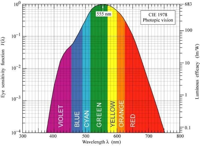
The lumen (lm) serves as the photometric equivalent of the watt (W), adjusted to match the eye’s response. According to the definition of the candela in SI units, there are $683$ lumens per watt for 555nm light that is propagating in a vacuum. Thus, the luminous intensity for light of a particular wavelength $\lambda$ is given by
\[I_\mathrm {v} ( \lambda ) = 683.002 \textrm{lm/W} \times V( \lambda ) \times I_\mathrm {e} ( \lambda ),\]where $I_\mathrm {v}(\lambda)$ is the luminous intensity, $I_\mathrm {e}(\lambda)$ is the radiant intensity and $V ( \lambda )$ is the photopic luminous efficiency function. For more general cases that the light source is not monochromatic, conversion from radiometric to photometric units might involve the integral of $\lambda$:
\[\Phi _{\mathrm {v} } = 683.002\ \mathrm { lm/W } \times \int _{0}^{\infty }{V}(\lambda )\Phi _{\mathrm {e} ,\lambda }(\lambda )\,\mathrm {d} \lambda,\]where
- $\Phi _{\mathrm {v} }$ is the luminous flux in $\textrm{lumen}$ ($\textrm{lm}$);
- $\Phi _{\mathrm {e}, \lambda}$ is the spectral radiant flux in $W / \textrm{nm}$;
- $V(\lambda)$ is the luminosity function, dimensionless;
- $\lambda$ is the wavelength in $\textrm{nm}$.
But since $V(\lambda)$ is given by a table of empirical values, it is possible to numerically approximate the integration.
Aside: Solid Angles
Radiometry concerns the measurement of energy across various regions of space, direction, and time. A pivotal unit of measurement within radiometry is the solid angle, which pertains to the concept of direction.
A solid angle $\Omega$ is defined as the ratio of the area $A$ of the segment of the sphere, given by the square of the radius $r$: $$ \Omega = \frac{A}{r^2} \; [\textrm{sr}] $$ where $\textrm{sr}$ denotes a dimensionless unit of solid angle, steradian, defined in the SI units. It is usually considered as the extension of radian in 2D to 3D space:
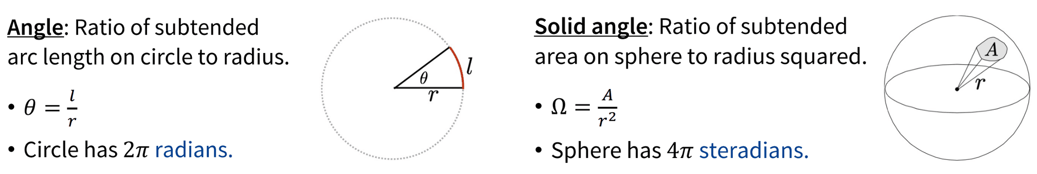
Intuitively, solid angles measure the extent to which an object covers the field of view from a specific point (apex), representing how large the object appears to an observer at that point. The point from which the object is viewed (viewing point) is called the apex of the solid angle, and the object is said to subtend its solid angle at that point. Therefore an object that blocks all rays from the apex would cover a number of steradians equal to the total surface area of the unit sphere, $4\pi$.
Solid Angle and Direction
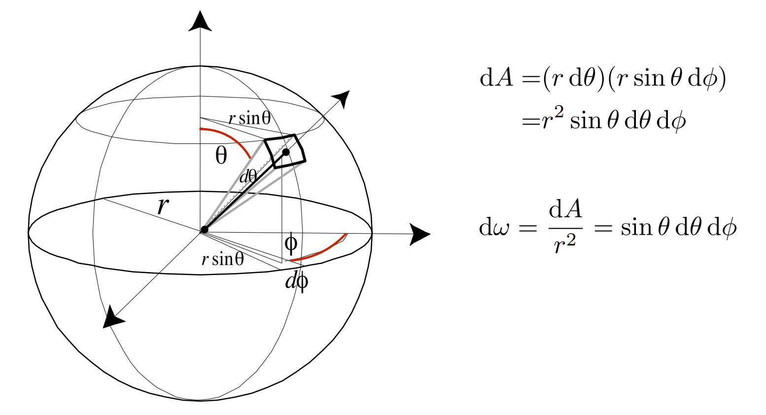
Considering directions (unit vectors) as being points on the unit sphere, solid angle serves as a means to quantify area on the unit sphere and consequently over the unit directions. In other words, the solid angle subtended by an object with area $A$ can be conceptualized as the set of (unit) direction vectors pointing toward that object. As elucidated in the next section, the solid angle $d\omega$ associated with the surface element of a sphere delimited by directions $(\theta, \phi)$, $(\theta + \mathrm{d}\theta, \phi)$, $(\theta, \phi + \mathrm{d}\phi)$, and $(\theta + \mathrm{d}\theta, \phi + \mathrm{d}\phi)$ is calculated as $d\omega =\sin \theta \,\mathrm{d}\theta \,\mathrm{d}\phi$. Hence, in radiometry and photometry, the unit direction to $(\theta, \phi)$ is denoted by $\omega$ and the solid angle $d\omega$ quantifies the notion of the area of a direction vector, i.e., a point on the sphere.
Differential Formula
For the integration, it is worth noting that there is a formula for the differential:
\[d\Omega =\sin \theta \,\mathrm{d}\theta \,\mathrm{d}\phi\]where $\theta$ is the colatitude (angle from the North Pole) and $\phi$ is the longitude. One can simply justify the formula with spherical coordinates, as illustrated in $\mathbf{Fig\ 6}$.
Here is an example.
The solid angle of a cone with its apex at the apex of the solid angle, and with apex angle $2 \theta$, is the area of a spherical cap on a unit sphere $$ \Omega = 2\pi (1 - \cos \theta) = 4\pi \sin^2 \frac{\theta}{2} $$
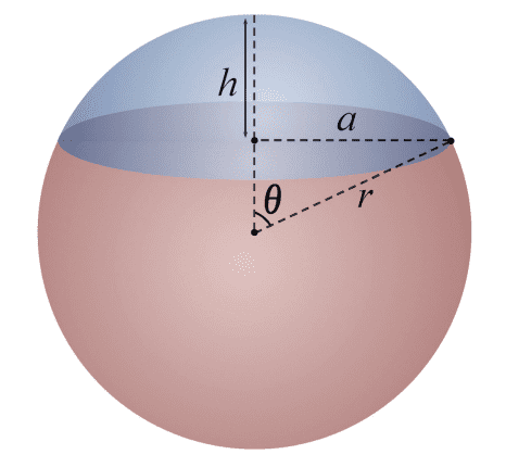
Note that for small $\theta \ll 1$ such that $\cos \theta \approx 1 - \frac{\theta^2}{2}$, the result reduces to the area of circle $\pi \theta^2$.
$\mathbf{Proof.}$
The calculation entails nothing more than computing the following double integral using the unit surface element in spherical coordinates:
\[\begin{aligned} \int_{\text{spherical cap}} d\Omega & = \int_{0}^{2\pi} \int_0^{\theta} \sin \theta^\prime \; \mathrm{d}\theta^\prime \; \mathrm{d}\phi \\ & = 2\pi \int_0^\theta \sin \theta^\prime \; \mathrm{d}\theta^\prime \\ & = 2\pi \left[ - \cos \theta \right]_{0}^\theta \\ & = 2 \pi (1 - \cos \theta). \end{aligned}\] \[\tag*{$\blacksquare$}\]Basic Radiometry (photometry) Units
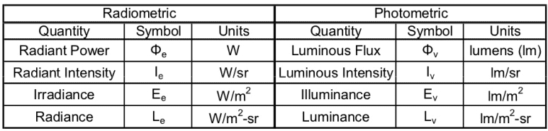
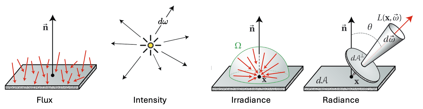
There are four radiometric quantities crucial to rendering: flux, intensity, irradiance and radiance.
They can each be derived from energy by successively taking limits over time, area, and directions.
The radiant (luminous) energy is the energy of electromagnetic radiation measured in units of Joules, denoted by the symbol $Q$ and defined by $$ Q = \frac{hc}{\lambda} \; [\mathrm{J} = \text{Joule}]. $$ where $Q$ is the energy carried by a photon at wavelength $\lambda$, $c = 299,472,458\textrm{m/s}$ is the speed of light, and $h \approx 6.626 \times 10^{-34} \textrm{m}^2 \textrm{kg/s}$ is Planck’s constant.
And as mentioned, all radiometric quantities have counterparts in photometry. Hence, photometric qunatities will be introduced simulatenously with radiometric quantities, denoted with parentheses.
Radiant (Luminous) Flux
The radiant (luminous) flux is often used to describe the radiation power output of the light source such as light bulb, or the radiation power received by an optical instrument.
The radiant (luminous) flux, or radiant (luminous) power is the total amount of energy passing through a surface or region of space per unit time: $$ \Phi = \lim_{\Delta t \to 0} \frac{\Delta Q}{\Delta t} = \frac{\mathrm{d}Q}{\mathrm{d}t} \; [\mathrm{W} = \text{Watt} = \mathrm{J/sec}] ([\textrm{lm} = \textrm{lumen}]) $$
Note that given flux $\Phi(t)$ as a function of time, the total energy is obtained by
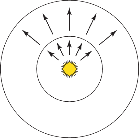
\[Q = \int_{t_1}^{t_2} \Phi(t) \; dt.\]$\mathbf{Fig\ 10}$ shows the flux from a point light source measured by the total amount of energy passing through imaginary spheres around the light. Note that the total amount of flux measured on either of the two spheres is the same, although less energy is passing through any local part of the large sphere than the small sphere, the greater area of the large sphere means that the total flux is the same.
Radiant (Luminous) Intensity
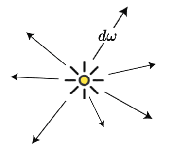
Consider an infinitesimal light source emitting photons. If we center this light source within the unit sphere, we can compute the angular density of emitted power, which is called intensity, denoted by $I$.
The radiant (luminous) intensity is defined by the power (flux) per unit solid angle emitted by a point light source. $$ I (\omega) = \lim_{\Delta \omega \to 0} \frac{\Delta \Phi}{\Delta \omega} = \frac{\mathrm{d} \Phi}{\mathrm{d} \omega} \left[ \frac{\textrm{W}}{\textrm{sr}} \right] \left(\left[ \frac{\textrm{lm}}{\textrm{sr}} = \textrm{cd} = \textrm{candela} \right]\right) $$ where $\textrm{sr}$ denotes steradian.
Conversely, given intensity as a function of direction $\omega$, we can integrate over a range of $\omega$ to compute the flux:
\[\Phi = \int_{\Omega} I (\omega) \; \mathrm{d}\omega\]Irradiance (Illuminance)
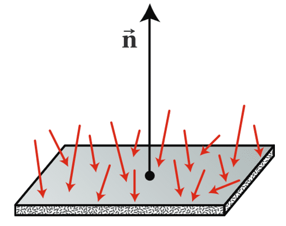
The measurement of flux necessitates consideration of the area over which photons per time (flux) are being measured. Given a finite area $A$, we can define the average density of power, $\Phi$, over the area as $E = \Phi / A$. This quantity is either irradiance (illuminance) ($E$), the area density of flux arriving at a surface, or radiant exitance, which also called radiosity (luminosity), the area density of flux leaving a surface. (The term irradiance is occasionally used to describe flux leaving a surface also.) It’s important to note that it denotes the direction-independent density of the light energy arriving at a surface from all directions.
The irradiance (illuminance) is defined by the power (flux) per unit area incident on a surface point $\mathrm{p}$: $$ E(\mathrm{p}) = \lim_{\Delta A \to 0} \frac{\Delta \Phi (\mathrm{p})}{\Delta A} = \frac{\mathrm{d} \Phi (\mathrm{p})}{\mathrm{d}A} \; \left[\frac{W}{m^2} \right] \left( \left[\frac{\textrm{lm}}{m^2}=\textrm{lux} \right]\right) $$
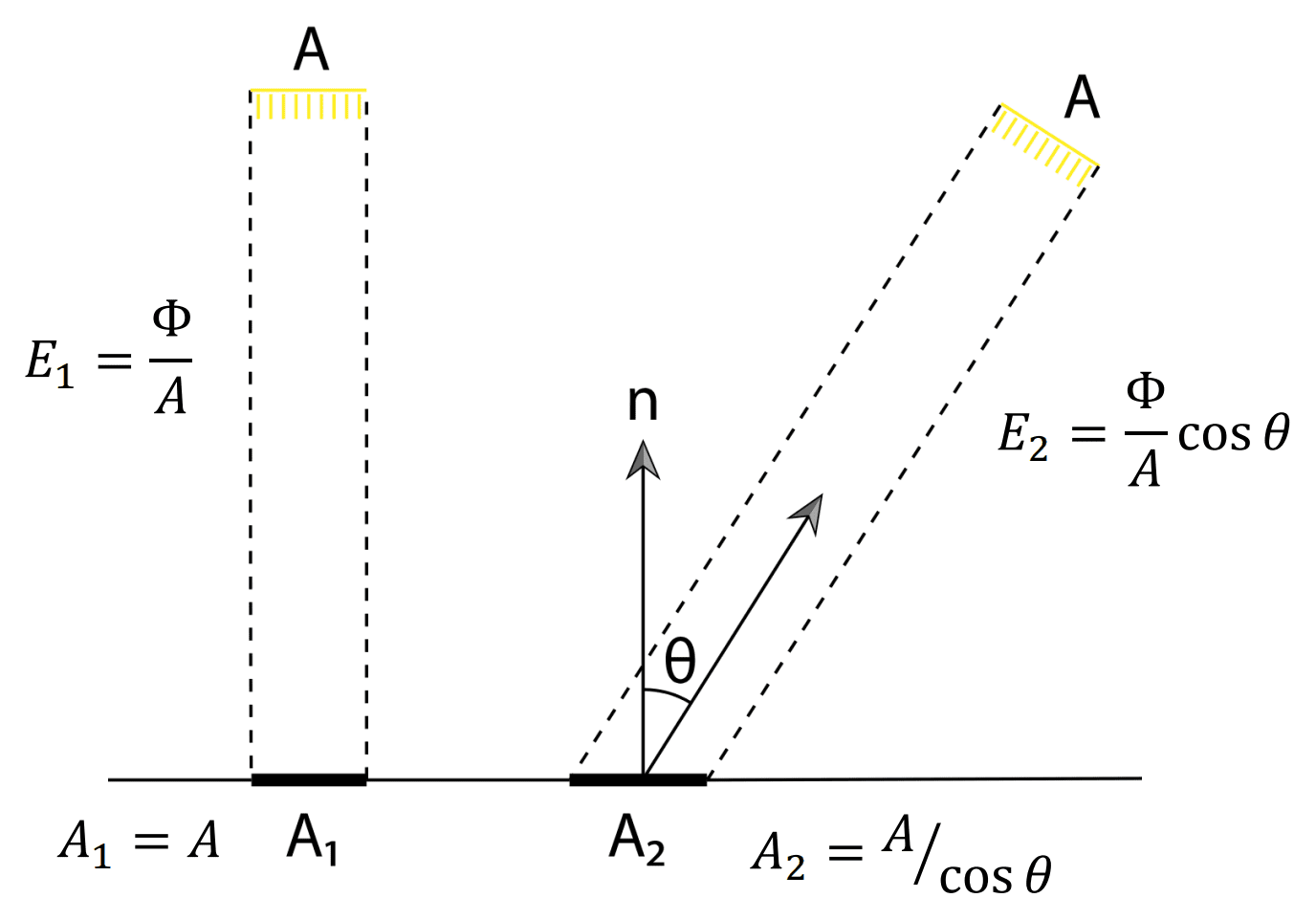
One of the pivotal concepts in rendering concerning irradiance is Lambert’s cosine law:
Irradiance at surface is proportional to cosine of angle, $\theta$, between light direction and surface normal. This phenomenon arises from the fact that illumination spans a greater area at larger incident angles.
Radiance (Luminance)
Irradiance provides us with the differential power per differential area at a point $\mathrm{p}$, i.e. the power arriving/leaving the point $\mathrm{p}$ toward all directions, yet it does not discern the directional distribution of power. And radiance (luminance) is defined by the solid angle density of irradiance (illuminance) to quantify the irradiance with respect to the direction:
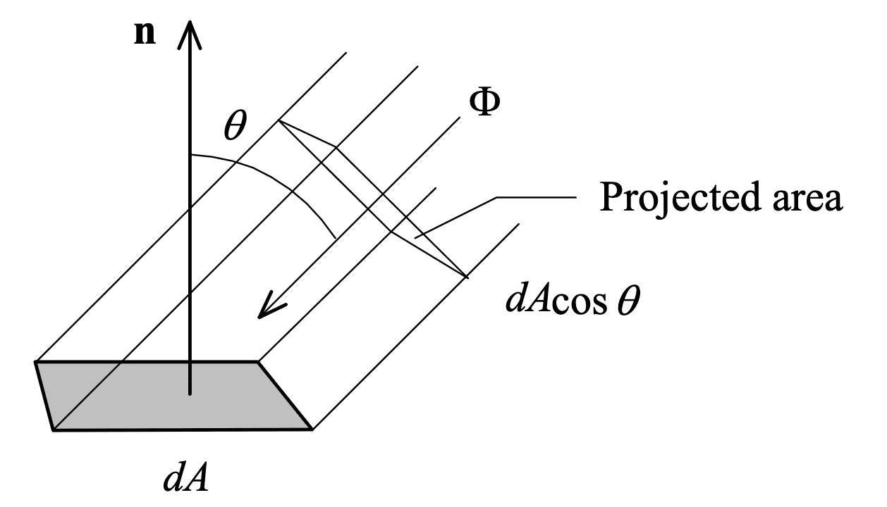
\[L (\mathrm{p}, \omega) = \lim_{\Delta \omega \to 0} \frac{\Delta E_{\omega} (\mathrm{p})}{\Delta \omega } = \frac{\mathrm{d} E_{\omega} (\mathrm{p})}{\mathrm{d} \omega} \; \left[ \frac{\textrm{W}}{\textrm{sr} \cdot \mathrm{m}^2} \right] \left( \left[ \frac{\textrm{lm}}{\textrm{sr} \cdot \mathrm{m}^2} = \frac{\textrm{cd}}{\mathrm{m}^2} = \textrm{nit} \right] \right)\]where $E_\omega$ denotes irradiance (illuminance) at the surface that is perpendicular to the direction $\omega = (\theta, \phi)$. For intuition, imagine ray of light arriving at or leaving a point on a surface in a perpendicular direction. Then, radiance simply indicates the infinitesimal amount of radiant flux contained in this ray. More generally, if the ray and the normal of surface that a point lies on is not parallel, the cross-sectional area of the ray is $\mathrm{d}A \cos \theta$, where $\theta$ is the angle between the ray and the surface normal.
Therefore, we define the radiance as follows:
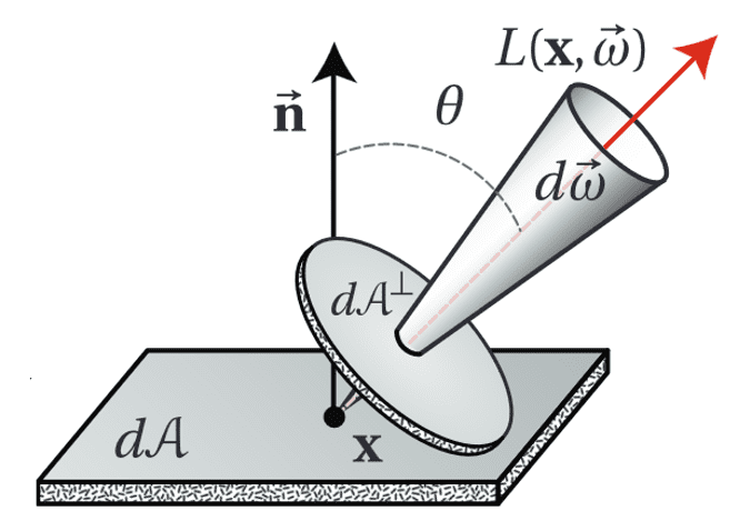
The radiance (luminance) is defined by the power (flux) emitted, reflected, transmitted or received by a surface point $\mathrm{p}$, per unit solid angle, per unit projected area: $$ L (\mathrm{p}, \omega) = \frac{\mathrm{d}^2 \Phi (\mathrm{p}, \omega)}{\mathrm{d} \omega \, \mathrm{d}A^\perp} = \frac{\mathrm{d}^2 \Phi (\mathrm{p}, \omega)}{\mathrm{d} \omega \, \mathrm{d}A \cos \theta} \; \left[ \frac{\textrm{W}}{\textrm{sr} \cdot \mathrm{m}^2} \right] \left( \left[ \frac{\textrm{lm}}{\textrm{sr} \cdot \mathrm{m}^2} = \frac{\textrm{cd}}{\mathrm{m}^2} = \textrm{nit} \right] \right) $$ where $\mathrm{d}A^\perp$ is the projected area of $\mathrm{d}A$ on a hypothetical surface perpendicular to the direction $\omega = (\theta, \phi)$.
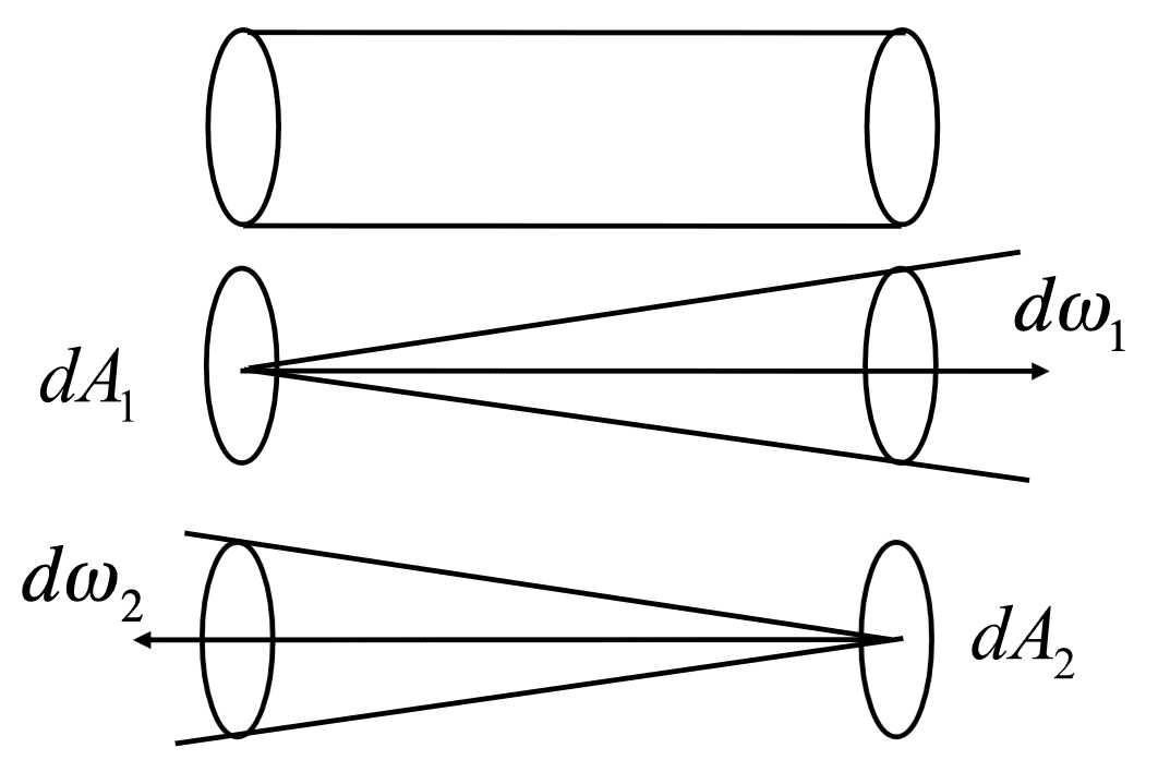
Among all previous radiometric quantities, radiance will be the most extensively utilized throughout the remainder of the book, as radiance derives all other values through integrals of radiance over areas and directions. Another advantageous property of radiance is its constancy along rays traversing empty space, which is known as conservation of radiance. This renders radiance a natural quantity to compute with ray tracing:
\[L_{\textrm{leave}} \, d\omega_{\textrm{leave}} \, \mathrm{d}A_{\textrm{leave}} = L_{\textrm{arrive}} \, d\omega_{\textrm{arrive}} \, \mathrm{d}A_{\textrm{arrive}} \\ \textrm{Total flux leaving one side} = \textrm{Total flux arriving other side}\]
Moreover, radiance is most directly and intimately related to the perceived brightness of colors by the human eye and is therefore the crucial quantity that must be computed for each pixel in a rendered image.
Incident & Exitant Radiance
Across surface boundaries, the radiance function $L$ generally shows discontinuity since the light physically interacts with surfaces in the scene. In the most extreme case of a fully opaque surface (e.g., a mirror), the radiance function slightly above and slightly below a surface could be completely unrelated. Consequently, it is obvious to consider one-sided limits at the discontinuity to differentiate between the radiance function just above and below of surface:
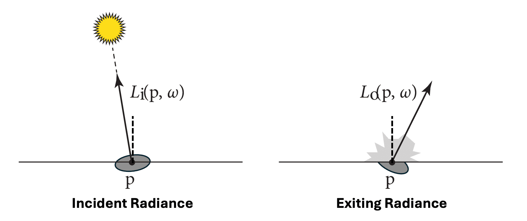
\[L^+ (\mathrm{p}, \omega) = \lim _{t \to 0^+} L (\mathrm{p} + t \mathbf{n}_p, \omega) \\ L^- (\mathrm{p}, \omega) = \lim _{t \to 0^-} L (\mathrm{p} + t \mathbf{n}_p, \omega) \\\]where \(\mathbf{n}_\mathrm{p}\) is the surface normal at $\mathrm{p}$. However, consistently tracking one-sided limits can become unnecessarily cumbersome. Instead, distinguish between two types of radiance arriving at the point $L_\mathrm{i} (\mathrm{p}, \omega)$ (e.g., due to illumination from a light source), termed incident surface radiance, and radiance departing that point $L_\mathrm{o} (\mathrm{p}, \omega)$ (e.g., due to reflection from a surface), termed exiting surface radiance.
The incident radiance $L_\mathrm{i}$ is defined by the irradiance per unit solid angle arriving at the surface point $\mathrm{p}$: $$ L_\mathrm{i} (\mathrm{p}, \omega) = \frac{\mathrm{d} E(\mathrm{p})}{\mathrm{d} \omega \cos \theta} $$ The exiting radiance $L_\mathrm{o}$ is defined by the intensity per unit projected area leaving at the surface point $\mathrm{p}$: $$ L_\mathrm{o} (\mathrm{p}, \omega) = \frac{\mathrm{d}I(\omega)}{\mathrm{d} A \cos \theta} $$
Therefore, it is possible to represent one-sided limits with more intuitive concepts incident and exitant radiance functions:
\[\begin{aligned} & L_{\mathrm{i}}(\mathrm{p}, \omega)= \begin{cases}L^{+}(\mathrm{p},-\omega), & \omega \cdot \mathbf{n}_{\mathrm{p}}>0 \\ L^{-}(\mathrm{p},-\omega), & \omega \cdot \mathbf{n}_{\mathrm{p}}<0\end{cases} \\ & L_{\mathrm{o}}(\mathrm{p}, \omega)= \begin{cases}L^{+}(\mathrm{p}, \omega), & \omega \cdot \mathbf{n}_{\mathrm{p}}>0 \\ L^{-}(\mathrm{p}, \omega), & \omega \cdot \mathbf{n}_{\mathrm{p}}<0 .\end{cases} \end{aligned}\]These two quantities measure distinct sets of photon events; incident radiance quantifies photons just before they arrive at a surface, while exitant radiance measures the photons leaving. Hence, in general
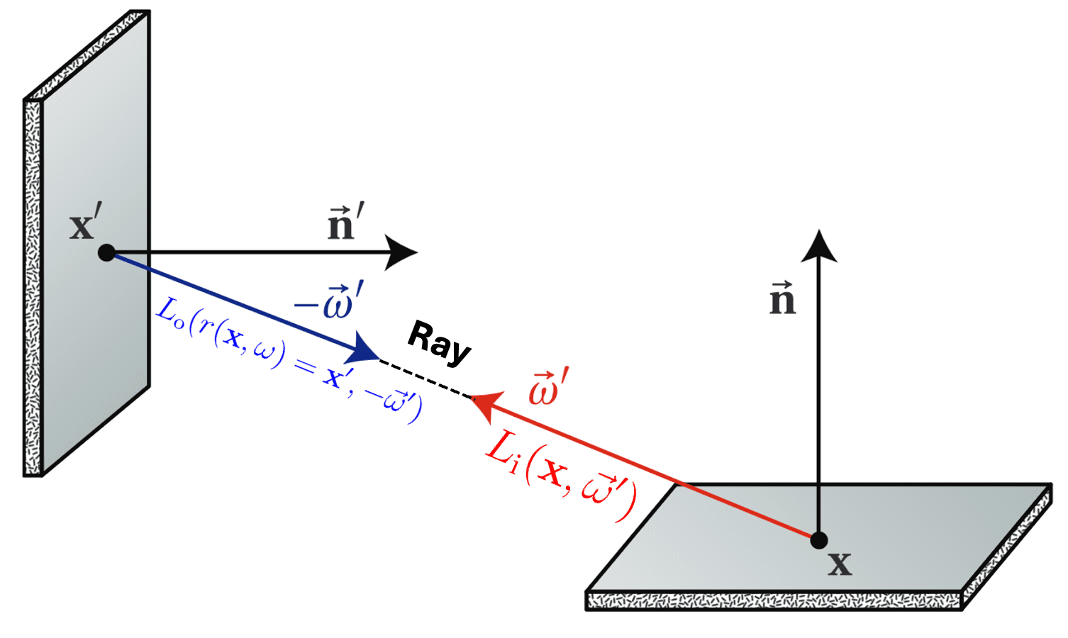
\[L_\mathrm{i} (\mathrm{p}, \omega) \neq L_\mathrm{o} (\mathrm{p}, \omega)\]However, in a vacuum, photons propagate unhindered. Consequently, all the radiance incident at a point from direction $\omega$ persists as exitant radiance in direction $-\omega$. Thus, radiance remains constant until it encounters a surface. This observation leads us to estabilish a simple, but useful connection between the incident and exitant radiance functions across two disparate points. To facilitate this, we introduce the ray casting function $r$:
\[r ( \mathbf{x}, \omega ) = \mathbf{x}^\prime\]where $\mathbf{x}^\prime$ denotes the point on the nearest surface to $\mathbf{x}$ in the direction of $\omega$. In scenarios where the space between surfaces constitutes a vacuum, radiance remains constant along straight trajectories, i.e. ray. This implies that the incident radiance at a point $\mathbf{x}$ from direction of $\omega$ equates to the outgoing radiance from the closest visible point $r(\mathbf{x}, \omega)$ in that direction:
\[L_{\textrm{i}}(\mathbf{x}, \omega) = L_{\textrm{o}} (r(\mathbf{x}, \omega), -\omega)\]
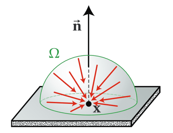
Here is an example of calculating irradiance with incident radiance.
From the definition of incident radiance, it is now possible to compute flux per unit area on surface occured by incoming light from all directions: $$ E(\mathrm{p}) = \int_{H^2} \mathrm{d}E (\mathrm{p}, \omega) = \int_{H^2} L_{\textrm{i}} (\mathrm{p}, \omega) \cos \theta \; \mathrm{d} \omega $$ where $\int_H^2$ denotes the integration of solid angles $\mathrm{d} \omega$ all over hemisphere $H^2$ and $$ dE (\mathrm{p}, \omega) = L_{\textrm{i}} (\mathrm{p}, \omega) \cos \theta \; \mathrm{d} \omega $$ is the differential irradiance, which indicates the contribution to irradiance from light arriving from direction $\omega$. As an example, by assuming the uniform hemispherical light, i.e. $L_{\textrm{i}} (\mathrm{p}, \omega) = L$ for some constant, we obtain $$ \begin{aligned} E(\mathrm{p}) & = \int_{H^2} L \cos \theta \; d\omega \\ & = L \int_0^{2\pi} \int_0^{\frac{\pi}{2}} \cos \theta \sin \theta \; \mathrm{d}\theta \; \mathrm{d}\phi \\ & = L \int_0^{2\pi} \int_0^{\frac{\pi}{2}} \frac{\sin 2\theta}{2} \; \mathrm{d}\theta \; \mathrm{d}\phi \\ & = L \cdot 2\pi \left[ - \frac{\cos 2\theta}{4} \right]_0^{\frac{\pi}{2}} \\ &= L \pi. \end{aligned} $$
BRDF (Bidirectional Reflectance Distribution Function)
With the definitions of incident and exiting radiance, our aim is to characterize how a surface reflects light, as we are concerned with rendering the appearance of 3D objects. At an intuitive level, for any incident light arriving from direction $\omega_{\textrm{i}}$, there exists some fraction scattered in a small solid angle near the outgoing reflected direction $\omega_{\textrm{r}}$. Various approaches could formalize such a concept, and the standard method is inspired by constructing a simple measurement device, depicted in the figure below:
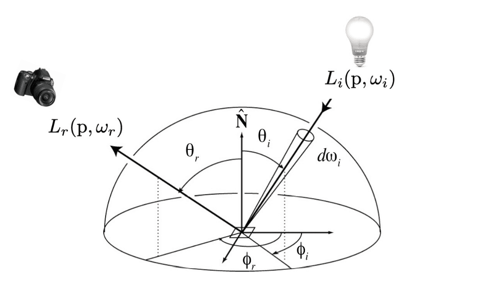
Firstly, from the definition of incident radiance, the infinitesimal irradiance $d E$ on the surface point $\mathrm{p}$ along the direction $ \omega_{\textrm{i}}$ from the single small source is given by
\[d E (\mathrm{p}, \omega_{\textrm{i}}) = L_{\textrm{i}} (\mathrm{p}, \omega_{\textrm{i}}) d\omega_{\textrm{i}} \cos \theta_{\textrm{i}}\]What we are interested in is the reflected radiation, denoted as $L_{\textrm{r}} (\mathrm{p}, \omega_{\mathrm{r}} = (\theta_{\mathrm{r}}, \phi_{\mathrm{r}}))$, along the direction $(\theta_{\mathrm{r}}, \phi_{\mathrm{r}})$. However, its important to note that other incident radiation, originating from other sources in other directions, may also be diffusely reflected (scattered) into the same reflected directions $(\theta_{\mathrm{r}}, \phi_{\mathrm{r}})$ along with that from the source under consideration.
Consequently, we calculate of the exiting radiance by integrating such contributions, i.e. the differential of exiting radiance $d L_{\mathrm{r}}$, generated by all the incident radiances based on our linearity assumption of lights. Thus $d L_{\mathrm{r}} \propto d E (\mathrm{p}, \omega_{\textrm{i}})$, leading to the following definition of BRDF:
The surface's bidirectional reflectance distribution function (BRDF) $f_r$ represents how much light is reflected into each outgoing direction $\omega_{\mathrm{r}}$, from each incoming direction $\omega_{\mathrm{i}}$ and is defined by $$ f_r\left(\mathrm{p}, \omega_{\mathrm{r}}, \omega_{\mathrm{i}}\right)=\frac{\mathrm{d} L_{\mathrm{r}}\left(\mathrm{p}, \omega_{\mathrm{r}}\right)}{\mathrm{d} E\left(\mathrm{p}, \omega_{\mathrm{i}}\right)}=\frac{\mathrm{d} L_{\mathrm{r}}\left(\mathrm{p}, \omega_{\mathrm{r}}\right)}{L_{\mathrm{i}}\left(\mathrm{p}, \omega_{\mathrm{i}}\right) \cos \theta_{\mathrm{i}} \mathrm{d} \omega_{\mathrm{i}}} \; \left[ \frac{1}{\textrm{sr}} \right] $$ Thus $$ L_{\mathrm{r}} \left(\mathrm{p}, \omega_{\mathrm{r}}\right) = \int_{H^2} f_r\left(\mathrm{p}, \omega_{\mathrm{r}}, \omega^{\prime}\right) L_{\mathrm{i}} \left(\mathrm{p}, \omega_{\mathrm{i}}\right) \cos \theta^{\prime} \mathrm{d} \omega^{\prime} $$ where $\int_{H^2}$ indicates the integration of solid angles all over the hemisphere.
Since two directions $(\omega_{\mathrm{r}}, \omega_{\mathrm{i}})$ are involved, the term “bidirectional” reflectance distribution function (BRDF) is used. From this definition, observe these results:
- BRDF is not bounded to the range $[0,1]$. Although the ratio $L_{\textrm{r}}$ to $L_{\textrm{i}}$ must fall within $[0,1]$ from the energy conservation assumption, the division by the cosine term in the denominator implies that a BRDF may possess values greater than $1$.
-
Reciprocity
The value of BRDF will remain unchanged if the incident and exitant directions are interchanged; i.e. for all pairs of directions $(\omega_{\mathrm{i}}, \omega_{\mathrm{r}})$, $$ f_r\left(\mathrm{p}, \omega_{\mathrm{r}}, \omega_{\mathrm{i}}\right) = f_r\left(\mathrm{p}, \omega_{\mathrm{i}}, \omega_{\mathrm{r}}\right) $$ This is also known as Helmholtz reciprocity or duality. Interpreting physically, this suggests that the sensitivity distribution with the observer at a given position equals to the distribution of reflected light with the source at the same position. -
Energy conservation
We assumed that the total energy of light reflected is less than or equal to the energy of incident light. And the radiant exitance is less than incident irradiance exactly when for all directions $\omega$ of incoming light $$ \int_{H^2} f_r\left(\mathrm{p}, \omega, \omega^{\prime}\right) \cos \theta^{\prime} \mathrm{d} \omega^{\prime} \leq 1 $$ It's important to highlight that this inequality is predicated on the assumption $L_{\mathrm{i}} (\omega_{\mathrm{i}}) = L \delta (\omega_{\mathrm{i}} = \omega)$, which represents a concentrated ray (laser) originating from $\omega$. This assumption is necessary condition for energy conservation within our geometric optics modeling, because any $L$ can be approximated by a linear combination of many $\delta$ functions and it is guaranteed that two different directions do not influence each other by the assumption of geometric optics.
Similar to BRDF, there exist various quantities that delineate the phenomena of light. For instance, BTDF (bidirectional transmission distribution function) elucidates how much light is transmitted when light interacts with a particular material. And BSSRDF (bidirectional scattering surface reflectance distribution function) characterizes scattering from materials exhibiting a substantial degree of subsurface light transport. We will delve into these concepts in subsequent posts.
Reference
[1] Huges et al. “Computer Graphics: Principles and Practice (3rd ed.)” (2013).
[2] Shirley et al. “Fundamentals of computer graphics” AK Peters/CRC Press, 2009.
[3] Matt Pharr, Wenzel Jakob, and Greg Humphreys, “Physically Based Rendering: From Theory To Implementation”
[4] lan Ashown. “Photometry and Radiometry” A Tour Guide for Computer Graphics Enthusiasts
[5] Stanford CS348B, Image Synthesis Techniques
[6] UC Berkeley CS184/284A, Computer Graphics and Imaging, “Measuring Light: Radiometry and Photometry”
[7] THORLABS, “Radiometric vs. Photometric Units”
[8] Wikipedia, “Candela”
[9] Wikipedia, “Luminous efficiency function”
[10] Wojciech Jarosz’s thesis
[11] Nicodemus, Fred (1965). “Directional reflectance and emissivity of an opaque surface”. Applied Optics. 4 (7): 767–775.
[12] Wojciech Jarosz, “Efficient Monte Carlo Methods for Light Transport in Scattering Media”, Ph.D. dissertation, UC San Diego, September 2008.
[13] Dutre, Philip, Philippe Bekaert, and Kavita Bala. Advanced global illumination. AK Peters/CRC Press, 2018.
Leave a comment