
[Graphics] Monte-Carlo Rendering
Probabilistic methods form the cornerstone of modern rendering techniques, particularly for estimating integrals, as solving the rendering equation necessitates computing an integral that is impossible to evaluate exactly except in the simplest scenes. In this post, we revisit fundamental Monte-Carlo methods, leveraging them to derive the single-sample estimate for an integral and the importance-weighted single-sample estimate for future discussions.
The Rendering Equation
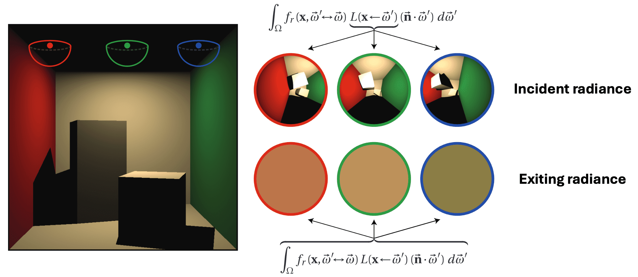
When assessing the brightness (exiting radiance) of point $\mathrm{p}$ on a surface, it relies on the incident radiance across the hemisphere above the point, and it can be visualized as a hypothetical “fisheye” view from $\mathrm{p}$. Subsequently, with BRDF, the exitant radiance at $\mathrm{p}$ is the integral of this value over the entire hemisphere. The entities on this hemisphere encompass both light sources and other surfaces, with their illumination computed in a similar manner. Consequently, this leads to a recursive correlation for the computation of illumination. For a visual aid, refer to $\mathbf{Fig\ 1.}$
Hemispherical Formulation
The key idea to construct the recursive equation is the energy conservation; at each particular position $\mathrm{p}$ and direction $\omega_{\mathrm{r}}$, the outgoing light $L_{\mathrm{r}} (\mathrm{p}, \omega_{\mathrm{r}})$ is the sum of the emitted light $L_{\mathrm{e}} (\mathrm{p}, \omega_{\mathrm{r}})$ and the reflected light. And the reflected light itself is the sum of the contributions from all directions of the incoming light $L_{\mathrm{i}} (\mathrm{p}, \omega_{\mathrm{i}})$ with BRDF $f_r (\mathrm{p}, \omega_{\mathrm{i}} , \omega_{\mathrm{r}})$
And the equation which mathematically describes this equilibrium is called the rendering equation, also known as light transport equation which defines the exiting radiance $L_{\mathrm{r}} (\mathrm{p}, \omega_{\mathrm{r}})$ of surface point $\mathrm{p}$ in outward direction $\omega_{\mathrm{r}}$ as the sum of the radiance emitted itself (if $\mathrm{p}$ is a point of a luminaire) and the reflected radiance:
\[\begin{aligned} \underbrace{L_{\mathrm{r}} (\mathrm{p}, \omega_{\mathrm{r}})}_\text{ outgoing } & = \underbrace{L_{\mathrm{e}} (\mathrm{p}, \omega_{\mathrm{r}})}_\text{ emitted } + \underbrace{\int_{H^2} f_r (\mathrm{p}, \omega_{\mathrm{i}} , \omega_{\mathrm{r}}) \cdot L_{\mathrm{i}} (\mathrm{p}, \omega_{\mathrm{i}}) \cdot (\omega_{\mathrm{i}} \cdot \vec{\mathbf{n}}_{\mathrm{p}}) \cdot d \omega_{\mathrm{i}}}_\text{ reflected } \\ & = L_{\mathrm{e}} (\mathrm{p}, \omega_{\mathrm{r}}) + \int_{H^2} f_r (\mathrm{p}, \omega_{\mathrm{i}} , \omega_{\mathrm{r}}) \cdot L_{\mathrm{i}} (\mathrm{p}, \omega_{\mathrm{i}}) \cdot \cos \theta_{\mathrm{i}} \cdot d \omega_{\mathrm{i}} \end{aligned} \tag 1\]where $f_r$ is the BRDF of the surface and $\theta_{\mathrm{i}}$ is the angle of incidence of $L_{\mathrm{i}}$. Since we have assumed that no participating media are present, radiance is constant along rays through the scene:
\[L_{\mathrm{i}} (\mathrm{p}, \omega_{\textrm{i}}) = L_{\mathrm{r}} (r(\mathrm{p}, \omega_{\textrm{i}}), - \omega_{\textrm{i}})\]where $r$ is the ray casting function that outputs the nearest surface point to $\mathrm{p}$ along the direction $\omega_{\textrm{i}}$ (see the previous post for detail). Discarding the subscripts from $L_{\textrm{r}}$ for brevity, we have
\[L (\mathrm{p}, \omega_{\textrm{r}}) = L_{\mathrm{e}} (\mathrm{p}, \omega_{\mathrm{r}}) + \int_{H^2} f_r (\mathrm{p}, \omega_{\mathrm{i}} , \omega_{\mathrm{r}}) \cdot L (r(\mathrm{p}, \omega_{\mathrm{i}}), -\omega_{\mathrm{i}}) \cdot \cos \theta_{\mathrm{i}} \cdot d \omega_{\mathrm{i}}\]where $L$ denotes the exitant radiance. The key observation to the above representation is that it now becomes the integral equation, i.e. there is only one quantity of interest, exitant radiance $L$ from points on surfaces. And this equation forms the recursive nature of global illumination, and is first introduced by Immel et al. 1986.
Surface Area Formulation
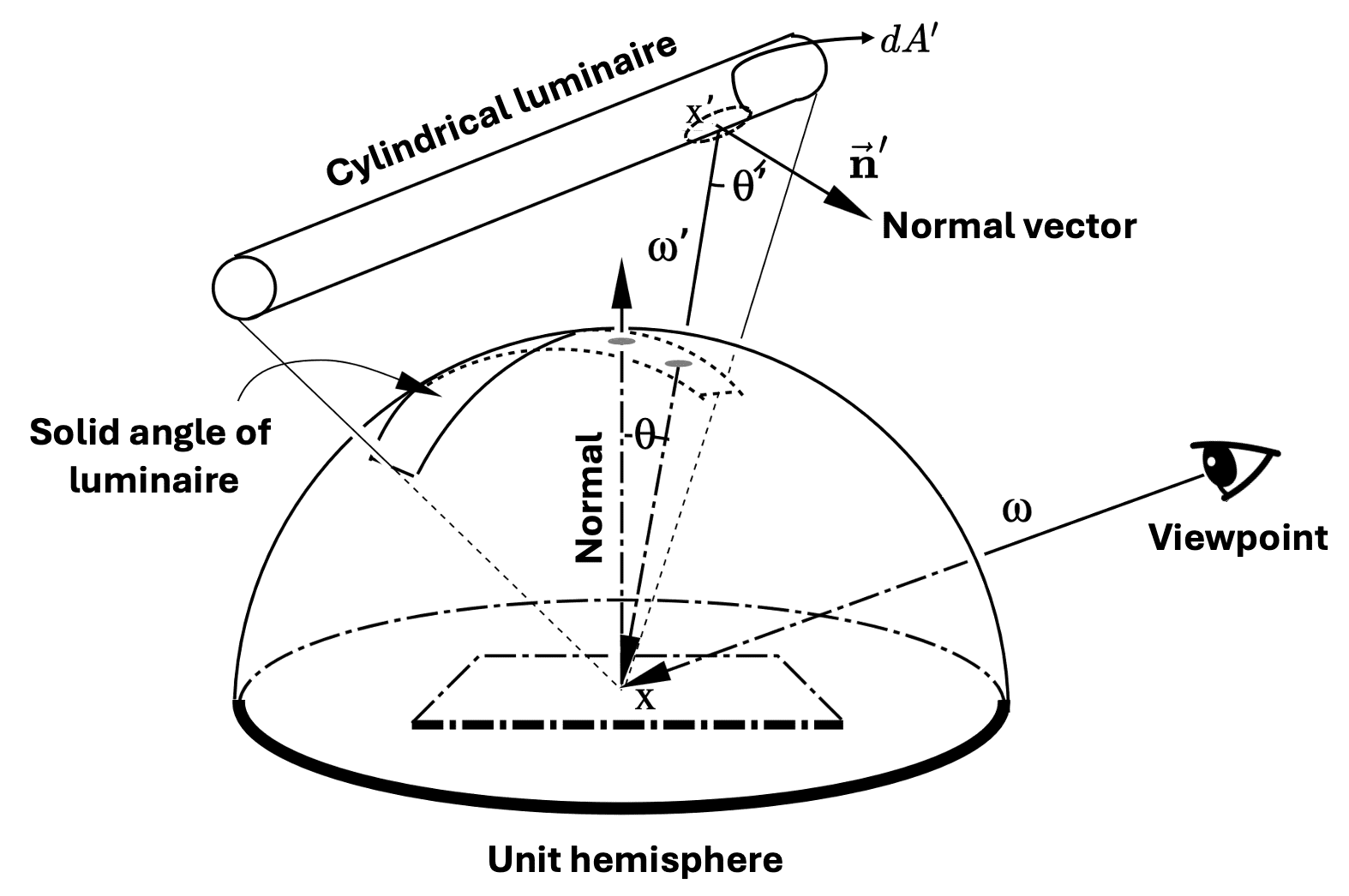
Simulatenously, Kajiya et al. 1986 introduced the rendering equation as an integration over points on the surfaces of the scene geometry. As shown in $\mathbf{Fig\ 2}$, we can consider projecting a differential area $dA^\prime$, which does not lie on the hemisphere, onto a spehere. Projecting this onto a sphere is equivalent to projecting it onto a plane which is perpendicular to the ray running from the center of the sphere to the center of $dA^\prime$. For sphere center $\mathbf{x}$ and a differential area $dA^\prime$ with the center $\mathbf{x}^\prime$ and surface normal $\vec{\mathbf{n}}^\prime$ we obtain the following differential equation:
\[d \omega^\prime = \frac{dA^\prime (\mathbf{x}^\prime) \cdot \cos \theta^\prime}{\lVert \mathbf{x} - \mathbf{x}^\prime \rVert^2} = \frac{dA^\prime (\mathbf{x}^\prime) \cdot (\vec{\mathbf{n}}^\prime \cdot - \omega^\prime)}{\lVert \mathbf{x} - \mathbf{x}^\prime \rVert^2} \tag 2\]
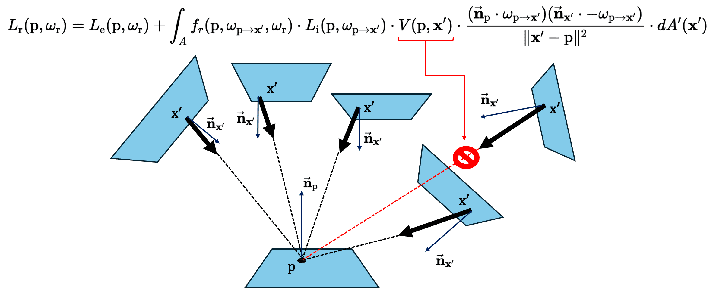
Note that the above discussion is only valid when $\mathbf{x}^\prime$ is a visible point at $\mathbf{x}$. Hence, we define the visibility function $V$ to discriminate the visible point at $\mathbf{x}$:
\[V(\mathbf{x}, \mathbf{x}^\prime) = \begin{cases} 1 & \quad \text{ if } \mathbf{x} \text{ and } \mathbf{x}^\prime \text{ are mutually visible } \\ 0 & \quad \text{ otherwise } \end{cases} \tag 3\]Finally, Kajiya’s area formulation of rendering equation can be done by performing a change of variable with the differential relation:
\[L_{\mathrm{r}} (\mathrm{p}, \omega_{\mathrm{r}}) = L_{\mathrm{e}} (\mathrm{p}, \omega_{\mathrm{r}}) + \int_{A}{f_r (\mathrm{p}, \omega_{\mathrm{p} \to \mathbf{x}^\prime} , \omega_{\mathrm{r}}) \cdot L_{\mathrm{i}} (\mathrm{p}, \omega_{\mathrm{p} \to \mathbf{x}^\prime}) \cdot V(\mathrm{p}, \mathbf{x}^\prime) \cdot \frac{(\vec{\mathbf{n}}_{\mathrm{p}} \cdot \omega_{\mathrm{p} \to \mathbf{x}^\prime}) (\vec{\mathbf{n}}_{\mathbf{x}^\prime} \cdot - \omega_{\mathrm{p} \to \mathbf{x}^\prime})}{\lVert \mathbf{x}^\prime - \mathrm{p} \rVert^2} \cdot d A^\prime (\mathbf{x}^\prime)} \tag 4\]where the integration domain $A$ extends to all surface points.
Monte-Carlo Rendering
There exist two main challenges that hinder solving the rendering equation:
- Inifinitely recursive
To obtain $L(\mathbf{x}, \omega)$, it requires $L(r(\mathbf{x}, \omega^\prime), -\omega^\prime)$ for all directions $\omega^\prime$ around the point $\mathbf{x}$. And again, for the calculation of each $L(r(\mathbf{x}, \omega^\prime), -\omega^\prime)$, it necessitates another exitant radiance recursively, and so forth. Consequently, the solution of the rendering equation for single point will depend on a huge number of other points and this inefficiency applies to all points on all surfaces in the environment. - Intractable integral
The integrand involving BRDF, radiance, and visibility are highly complex and often contain many discontinuities, rendering the integral intractable.
To circumvent these issues, the rendering equation is typically approximated using numerical integration. Several algorithms have been proposed in the literature to fully or partially solve the rendering equation, and these global illumination algorithms can be roughly be divided into two groups: Monte Carlo-based, and finite element method-based rendering (but also combining two methods are also possible and have been developed already).
- Finite element method-based Rendering
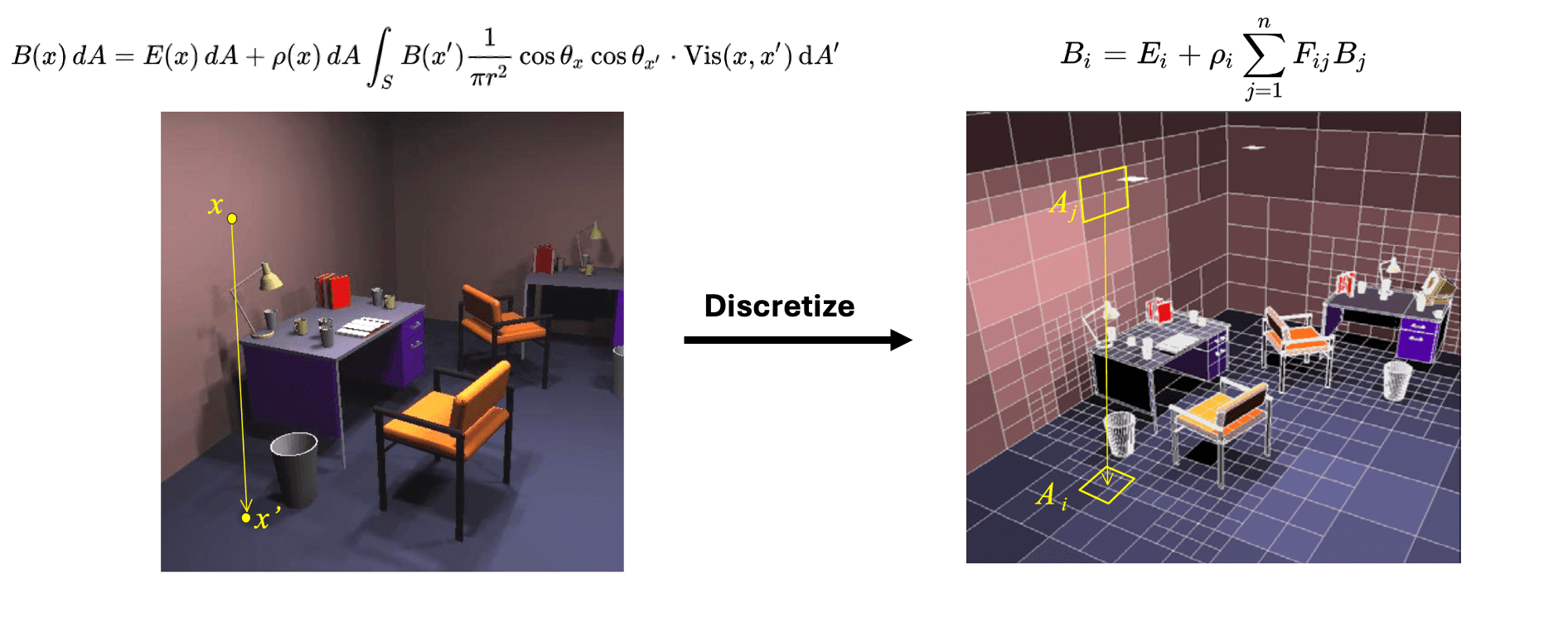
In computer graphics, finite element-based methods are typically referred t as radiosity methods. This approach involves discretizing the scene geometry into a collection of small patches, and these patches form the basis upon which the global illumination solution is derived. Specifically, the illumination computation is solved by reformulating the rendering integral equation as a linear system of equations that describes the radiosity $B$, the energy per unit area departing from the surface of each patch per discrete time interval-across all patches within the scene.
Nonetheless, radiosity-based methods typically demand substantial memory resourses and intricate implementation. Furthermore, scene subdivision is sensitive and thus fragile to the fidelity of the geometry model. Consequently, these methods are generally less practical to use for the complete rendering equation. Therefore, this post centers on Monte-Carlo rendering; for further insights into radiosity methods, refer to this Wikipedia and MIT 6.837 Fall ‘01: Radiosity v.s. Ray Tracing.
$\mathbf{Fig\ 4.}$ Visualization of radiosity method (MIT 6.837 Fall ‘01)
- Monte Carlo-based Rendering
In contrast, Monte-Carlo rendering leverages random sampling according to the given PDF $p$ in order to compute the integration in the rendering equation: $$ L (\mathrm{p}, \omega_{\textrm{r}}) \approx \frac{1}{N} \sum_{k=1}^N \left[ L_{\mathrm{e}} (\mathrm{p}, \omega_{\mathrm{r}}) + \frac{f_r (\mathrm{p}, \omega_k , \omega_{\mathrm{r}}) \cdot L (r(\mathrm{p}, \omega_k), -\omega_k)}{p(\omega_k)} \right] \text{ where } \omega_k \sim p (\omega_k) \tag 5 $$ However, we do not yet know the value of other exitant radiances $L (r(\mathrm{p}, \omega_k), -\omega_k)$. To compute the radiance, we compute a visible point $r(\mathrm{p}, \omega_k)$, from $\mathrm{p}$ toward $\omega_k$ direction and then recursively use another unbiased MC estimator $\widetilde{L} (r(\mathrm{p}, \omega_k), -\omega_k)$ of $L (r(\mathrm{p}, \omega_k), -\omega_k)$. This recursion process terminates when a ray intersects with a light source, establishing a light path from the light source to the viewpoint (eye). And the aformentioned process is the basic idea of path tracing that we will discuss in the future post.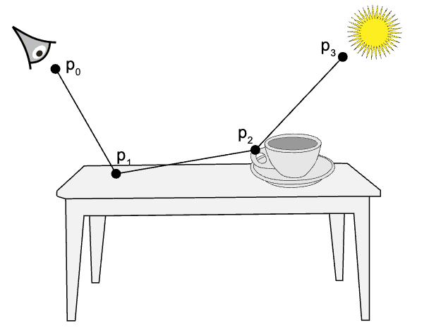
$\mathbf{Fig\ 5.}$ Visualization of path tracing (PBR Book)
Indeed, in graphics, Monte Carlo methods emerged independently. Their inception can be traced back to Appel et al. 1968 that utilized random particle tracing to compute images. Subsequently, Whitted et al. 1980 introduced ray tracing, which involves recursively evaluating surface appearance, and also proposed the notion of randomly perturbing viewing rays. These innovations led to the first comprehensive, unbiased Monte Carlo rendering algorithm known as path tracing, as proposed by Kajiya et al. 1986. They proposed the rendering equation, and recognized that this could be tackled by sampling paths. And over the ensuing years, numerous other algorithms have been devised for resolving the rendering equation using Monte Carlo methods. Below is the brief summary of some groundbreaking algorithms, borrowed from Shaohua Fan's Ph.D. dissertation.
$\mathbf{Table\ 1.}$ Monte Carlo algorithms for global illumination (Shaohua Fan)
Basic: Monte-Carlo Integration
In this section, we delve into the basics of Monte Carlo integration, a technique utilized to evaluate complex integral functions such as the rendering equation. Subsequently, in future posts, we will explore Monte Carlo-based ray tracing techniques, specialized methods for resolving rendering equations.
Monte Carlo integration operates on the premise that the definite integral of a given function can be approximated by sampling the function at multiple random positions within the integration domain. Since Monte Carlo can yield arbitrarily accurate results depending on the number of samples used, it has gained much importance in the field of computer graphics. Conceptually, Monte Carlo integration resembles integration by (deterministic) numerical quadrature, but the samples of Monte-Carlo chosen randomly instead of being distributed evenly across the integration domain. Notably, in higher dimensions, numerical quadrature becomes significantly less effective compared to Monte Carlo, as the requisite number of samples grows exponentially.
Monte-Carlo Estimation
Consider calculating a 1D integral $\int_a^b f(x) \; dx$. With independent uniform random variables $X_j \sim \mathcal{U}[a, b]$, the Monte-Carlo estimator $F_n$ is defined by
\[F_n = \frac{b-a}{n} \sum_{j=1}^n f(X_j) \tag 6\]where it is an unbiased estimator of the integral, i.e. $\mathbb{E}[F_n]$ is equal to the integral:
\[\begin{aligned} \mathbb{E}[F_n] & = \frac{b-a}{n} \sum_{j=1}^n \mathbb{E} \left[ f(X_j) \right] \\ & = \frac{b-a}{n} \sum_{j=1}^n \int_a^b f(x_j) \cdot \frac{1}{b-a} \; dx_j \\ & = \int_a^b f(x) \; dx \end{aligned} \tag 7\]from the assumption that $X_j \sim \mathcal{U}[a, b]$. And generally, for $N$-dimensional integral
\[\int_{a_N}^{b_N} \cdots \int_{a_2}^{b_2} \int_{a_1}^{b_1} f(x_1, x_2, \cdots, x_N) \; dx_1 dx_2 \cdots dx_N \tag 8\]we uniformly sample $n$ independent $X_j$ from the $N$-dimensional cude $\prod_{j=1}^N [a_j, b_j]$ and the pdf of $X$, denotes as $p(X)$ is then given by
\[p(X) = \prod_{j=1}^N \frac{1}{b_j - a_j} \tag 9\]Then the Monte-Carlo estimator is
\[\frac{\prod_{j=1}^N (b_j - a_j)}{n} \sum_{j=1}^n f(X_j) \tag {10}\]Extending to the Monte-Carlo estimator with non-uniform random samples is now straightforward and necessitates only small changes. With $n$ random samples $X_j \sim p(x)$ where $p$ is the pdf of arbitrary distribution, we define the Monte-Carlo estimator as
\[F_n = \frac{1}{n} \sum_{j=1}^n \frac{f(X_j)}{p(X_j)} \tag {11}\]but $p(x)$ must be non-zero for all $x$ where $f(x) \neq 0$. Again, it is an unbiased estimator of integral:
\[\begin{aligned} \mathbb{E}[F_n] & = \frac{1}{n} \sum_{j=1}^n \mathbb{E} \left[ \frac{f(X_j)}{p(X_j)} \right] \\ & = \frac{1}{n} \sum_{j=1}^n \int_a^b \frac{f(x_j)}{p(X_j)} \cdot p(x_j) \; dx_j \\ & = \int_a^b f(x) \; dx \end{aligned} \tag {12}\]Therefore, to approximate the given integral, the samples can be chosen with arbitrary distribution, regardless of the dimensionality of the integrand. And the convergence of Monte-Carlo estimator to the true value is typically guaranteed by the law of large numbers.
Error of Monte Carlo Estimators
Note that the estimator $F_n$’s are all unbiased; its expectation is equal to the integral. But one of the most important quantities for measuring the quality of estimator is variance, expectation of squared error:
\[\textrm{Var}[F] = \mathbb{E} [ (F - \mathbb{E}[F])^2 ] = \mathbb{E}[F^2] - \mathbb{E}[F]^2 \tag{13}\]Recall that if the variance of a sum of independent random variables $X_i$, just like the Monte-Carlo estimator $F_n$, is given by the sum of the individual random variables’ variances:
\[\textrm{Var} \left[ \sum_{j=1}^n X_j \right] = \sum_{j=1}^n \textrm{Var}[X_j] \tag{14}\]With this equation, we can easily derive the variance of $F_n$ with random samples from distribution $p$:
\[\textrm{Var}[F_n] = \textrm{Var}\left[ \frac{1}{n} \sum_{j=1}^n \frac{f(X_j)}{p(X_j)} \right] = \frac{1}{n^2} \sum_{j=1}^n \textrm{Var} \left[ \frac{f(X)}{p(X)} \right] = \frac{1}{n} \textrm{Var} \left[ \frac{f(X)}{p(X)} \right] = \mathcal{O} \left(\frac{1}{n} \right) \tag{15}\]Hence variance decreases linearly with the number of samples $n$. And since variance is squared error, the error in a Monte Carlo estimate therefore only goes down at a rate of $\mathcal{O} (n^{-1/2})$ in the number of samples.
Here is an example.
$\mathbf{Answer.}$
We have
\[\begin{aligned} \textrm{Var} [ F_1 ] & = \frac{\sigma^2}{n} \\ \textrm{Var} [ F_2 ] & = \frac{\sigma^2}{2n} \end{aligned}\]Since $F_1$ can take 3 times more samples during the same amount of time, with $3n$ samples, the variance of $F_1$ decreases to
\[\textrm{Var} [ F_1 ] = \frac{\sigma^2}{3n}\]Therefore, $F_1$ is better estimator than $F_2$. Likewise, we may define the efficiency $e$ of an estimator $F$ as follows:
\[e [F] = \frac{1}{\textrm{Var}[F] \cdot \mathcal{T}[F]}\]where $\mathcal{T}[F]$ is the computation time of the estimator $F$.
\[\tag*{$\blacksquare$}\]The actual error of the Monte Carlo estimator is still required to be determined and two theorems are popular to be used for this purpose. The first is Chebyshev’s inequality, which can be proved easily:
\[\mathbb{P} \left( \lvert F - \mathbb{E}[F] \rvert \geq \sqrt{\frac{\textrm{Var}[F]}{\varepsilon}}\right) \leq \varepsilon \tag{16}\]It asserts tha the probability that the estimator $F$ deviates from its expectation $\mathbb{E}[F]$ by an amount exceeding $\sqrt{\textrm{Var}[F]/\varepsilon}$ is less than $\varepsilon$ where $\varepsilon > 0$ is any arbitrary positive number. By substituting the variance of the Monte Carlo estimator, we derive:
\[\mathbb{P} \left( \left\vert F_n - \int_a^b f(x) \; dx \right\vert^2 \geq \frac{1}{n\varepsilon}\textrm{Var}\left[\frac{f(X)}{p(X)} \right]\right) \leq \varepsilon \tag{17}\]Hence, by discerning the variance of $f(X)/p(X)$ and selecting a specific probability $\varepsilon$, we can always compute a necessitated number of samples $n$ such that the probability of our estimator deviating from the integral is less than $\varepsilon$.
The second theorem utillized for assessing the error of Monte Carlo computations is the central limit theorem. This theorem posits that the Monte Carlo estimator will asymptotically (i.e. for $n \to \infty$) conform to a normal distribution.
Bias and Consistency
Clearly, not all estimators are necessarily equally good. Some may converge slower toward the desired value, some faster; likewise, the expectation of some estimators may not always be equal to the desired value, either. An estimator $F$ which expectation does NOT match the approximating quantity $\theta$ is called a biased estimator, i.e., the bias
\[\textrm{bias}(F, \theta) = \mathbb{E}[F] - \theta \tag{18}\]is non-zero. While it is more desirable to have an unbiased estimator, one should also consider the variance of the estimator as a factor of interest. A biased estimator with low variance is usually preferred to an unbiased one with high variance. Here is an example borrowed from Kalos and Whitlock, 1986.
$\mathbf{Answer.}$
For the first estimator, we have
\[\begin{aligned} \mathbb{E}[F_1] & = \frac{1}{n} \sum_{i=1}^n \mathbb{E}[X_i] = \frac{1}{2} \\ \textrm{Var}[F_1] & = \frac{1}{n^2} \sum_{i=1}^n \textrm{Var}[X_i] = \frac{1}{n^2} \frac{n}{12} = \mathcal{O}\left(\frac{1}{n} \right) \\ \end{aligned}\]For the second estimator, note that the cdf of $F_2$ is given by
\[\textrm{CDF}(x) = \mathbb{P}(F_2 \leq x) = \mathbb{P}(\max (X_1, \cdots, X_n) \leq 2x) = \begin{cases} 1 & \quad \text{ if } x > \frac{1}{2} \\ (2x)^n & \quad \text{ if } 0 < x \leq \frac{1}{2} \\ 0 & \quad \text{ if } x \leq 0 \end{cases}\]Therefore, the pdf of $F_2$ is given by
\[p(x) = \frac{d}{dx} (2x)^n = n2^n x^{n-1} \quad x \in \left[0, \frac{1}{2} \right]\]and
\[\begin{aligned} \mathbb{E}[F_2] & = n 2^n \int_0^{1/2} x^{n} \; dx = \frac{n}{2 (n+1)} \\ \mathbb{E}[F_2^2] & = n 2^n \int_0^{1/2} x^{n+1} \; dx = \frac{n}{4 (n+2)} \\ \textrm{Var}[F_2] & = \mathbb{E}[F_2^2] - \mathbb{E}[F_2]^2 = \frac{n}{4(n+1)^2(n+2)} = \mathcal{O}\left(\frac{1}{n^2} \right) \\ \end{aligned}\]Therefore, while $\mathbb{E}[F_2] \neq \frac{1}{2}$, i.e. biased estimator, it still converges to $\frac{1}{2}$ when $n \to \infty$. Moreover, $\textrm{Var}[F_2] = \mathcal{O} \left( n^{-2} \right)$, which converges much faster than $F_1$ as $n \to \infty$.
\[\tag*{$\blacksquare$}\]In many cases, it is challenging to find an unbiased estimator in general. Therefore, in such scenarios, a weaker constraint can be imposed; an estimator $F$ is called consistent if $F$ converges to $\theta$ with probability $1$ as the number of samples $n \to \infty$, i.e.
\[\mathbb{P} \left[ \lim_{n \to \infty} F (X_1, \cdots, X_n) = \theta \right] = 1 \tag{19}\]As an example, $F_2$ in the previous example is the consistent estimator of mean.
Sampling and Variance Reduction
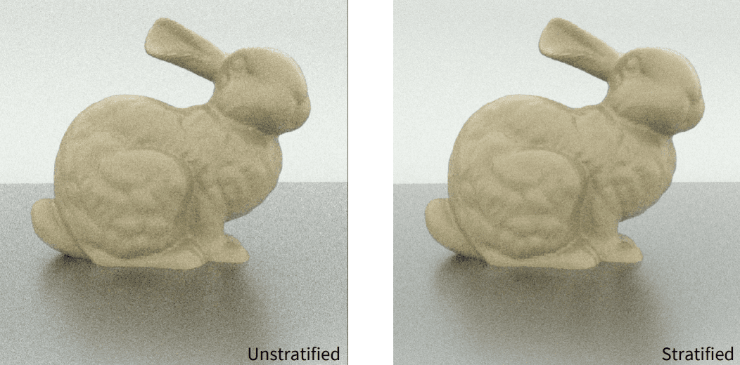
The downside of Monte-Carlo techniques is variance, which manifests itself as high-frequency noise in rendered images. Consequently, a wide variety of variance reduction methods have been developed with the aim of reducing the required number of samples to converge, while synthesizing a high quality image. In this section, we investigate two very widespread and widely discussed sampling strategies for variance reduction, called stratified and importance sampling.
Stratified Sampling
Stratified sampling tries to address the problem that samples are often chosen unevenly from the integration domain, thus resulting in “clumping”. It decomposes the integration domain $\Lambda$ into $m$ disjoint subdomains \(\{ \Lambda_i \}_{i=1}^m\) (called stratum) and approximate each resulting integral separately.
\[\int_{\Lambda} f(x) \; dx = \sum_{i=1}^m \int_{\Lambda_i} f(x) \; dx \tag{20}\]This method does indeed reduce variance; with total number of samples $n$, draw $n_i = v_i n$ samples \(\{ X_{i, j} \}_{j = 1}^{n_i}\) from each $\Lambda_i$, according to densities $p_i$ inside each stratum where $v_i \in [0, 1]$ is the fractional volume of $i$-th stratum $\Lambda_i$. Within a single stratum $\Lambda_i$, then the overall estimate is $F = \sum_{i=1}^m v_i F_i$ where $F_i$ is the Monte-Carlo estimate of $\int_{\Lambda_i} f(x) \; dx$, i.e. $F_i = \frac{1}{n_i} \sum_{j=1}^{n_i} f(X_{i, j})/p_i (X_{i, j})$.
For simple analysis, assume that $\Omega = [0, 1]^s$ and that $p_i$ is simply the constant function on $\Omega_{i}$. This leads to an estimate of the form
\[\begin{aligned} F & =\sum_{i=1}^m v_i F_i \\ \text { where } \quad F_i & =\frac{1}{n_i} \sum_{j=1}^{n_i} f\left(X_{i, j}\right) . \end{aligned}\]Then by letting $\mu_i = \mathbb{E}[f(X_{i, j})]$ and $\sigma_i^2 = \textrm{Var}[f(X_{i,j})]$, we obtain the variance of the overall estimator $F$
\[\begin{aligned} \textrm{Var}[F] & = \textrm{Var}\left[ \sum_{i=1}^m \frac{v_i}{n_i} \sum_{j=1}^{n_i} f(X_{i, j}) \right] \\ & = \sum_{i=1}^m \frac{v_i^2}{n_i^2} \sum_{j=1}^{n_i} \textrm{Var} [f(X_{i, j})] \\ & = \sum_{i=1}^m \frac{v_i^2 \sigma_i^2}{n_i} = \frac{1}{n} \sum_{i=1}^m v_i \sigma_i^2 \end{aligned} \tag{21}\]To compare this result to the Monte-Carlo estimator without stratification, denoted as $F_U$, observe that unstratified sampling is equivalent to
- sampling a random stratum $\Lambda_i$ according to the discrete probability $v_i$, i.e., $p(\Lambda_i) = v_i$ and then
- sampling $X_{ij}$ conditionally within $\Lambda_i$, i.e. $p(X_{ij} \vert \Lambda_i) = p_i (X_{ij})$
In this sense, from the law of total variance, i.e., $\textrm{Var} [f(X_{i, j})] = \mathbb{E}[\textrm{Var} [ f(X_{i, j}) \vert \Lambda_i]] + \textrm{Var}[\mathbb{E}[f(X_{i, j}) \vert \Lambda_i]]$, and we have
\[\begin{aligned} \mathbb{E}[f(X_{i, j}) \vert \Lambda_i] & = \int f(X_{i, j}) \cdot p(X_{ij} \vert \Lambda_i) \; dx = \int_{\Lambda_i} f(X_{i, j}) \cdot p_i (X_{ij}) = \mu_i \\ \textrm{Var}[\mathbb{E}[f(X_{i, j}) \vert \Lambda_i]] & = \mathbb{E}[ (\mathbb{E}[f(X_{i, j}) \vert \Lambda_i] - \mathbb{E}[\mathbb{E}[f(X_{i, j}) \vert \Lambda_i]])^2 ] \\ & = \mathbb{E} \left[ \left( \mu_i - \sum_{i=1}^{m} v_i \mu_i \right)^2 \right] = \sum_{k=1}^m v_k \cdot \left( \mu_k - \sum_{i=1}^{m} v_i \mu_i \right)^2 \end{aligned} \tag{22}\]Thus we obtain:
\[\textrm{Var} [F_U] = \frac{1}{n} \left[ \sum_{i=1}^m v_i \sigma_i^2 + \color{red}{\underbrace{\sum_{i=1}^m v_i (\mu_i - \mu)^2}_{\textrm{Non-negative value!}}} \right] \geq \textrm{Var} [F] \tag{23}\]This result implies that pre-defining the number of sample $n_i$ in each partition $\Lambda_i$ is less risky than totally random sampling over the entire domain $\Lambda$.
The main drawback of stratified sampling is the curse of dimensionality. Complete stratification in $D$ dimensions with $S$ strata per dimension necessitates $S^D$ samples, which swiftly becomes impractical. Therefore, it primarily proves effective for low-dimensional integration problems where the integrand is reasonably well-behaved. If the dimension of integral is high, or if the integrand has singularities or rapid oscillations in value (e.g. a texture with fine details), then the efficacy of stratified sampling diminishes significantly.
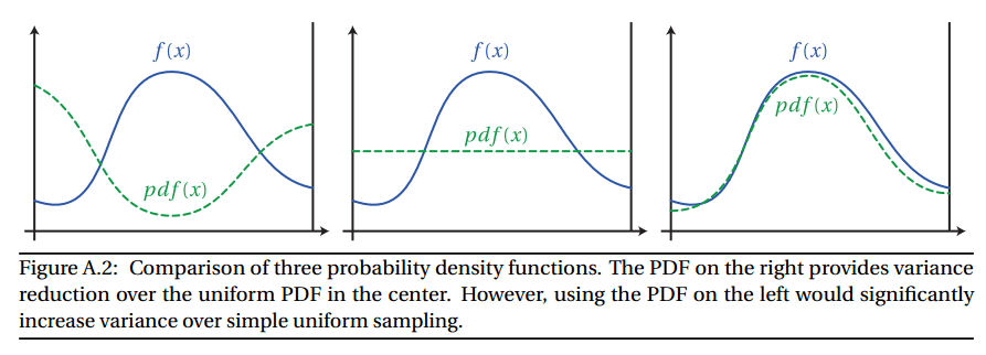
Importance Sampling
From the equation $\textrm{(15)}$, when computing an integral using Monte Carlo, the variance of the estimator depends only on the number of samples $n$, $f(X)$ and $p(X)$. Since $f (x)$ cannot be influenced, this leaves us with two ways of modifying the variance:
- Increasing or decreasing the number of samples.
- Choosing a certain sampling probability density function $p(X)$.
Hence, we want to find a $p(X)$ such that the variance is as low as possible (ideally, the variance should be zero, yielding a perfect estimator). This can be done by using Cauchy-Schwartz inequality.
$\mathbf{Proof.}$
Note that $c = \int_a^b \lvert f(x) \rvert \; dx$. Let
\[g_p (X) = \frac{f(X)}{p(X)}\]where $X \sim p$. It suffices to show that $\textrm{Var} [g_{\bar{p}}(X)] \leq \textrm{Var} [g_p(X)]$ since the variance of the sum of independent random variables is equal to the sum of the variances of the random variables. Note that for any density $p$, $\mathbb{E}[g_p (X)] = \int_a^b f(x) \; dx$. Then, for any density $p$,
\[\begin{aligned} \textrm{Var} [g_{\bar{p}} (X)] - \left(\int_a^b f(x) \; dx\right)^2 & = \mathbb{E}[ g_\bar{p}(X)^2 ] = \int \frac{f^2(X)}{\bar{p}(X)} \; dx \\ & = c \int \lvert f(x) \rvert \; dx \\ & = \left( \int \lvert f(x) \rvert \; dx \right)^2 \\ & = \left( \int \frac{\lvert f(x) \rvert}{p(x)} p(x) \; dx \right)^2 \\ & \leq \int \frac{f(x)^2}{p^2(x)} p(x) \; dx \\ & = \int \frac{f(x)^2}{p(x)} \; dx \\ & = \textrm{Var} [g_{p} (X)] - \left(\int_a^b f(x) \; dx\right)^2 \end{aligned}\]where the inequality is derived from the Cauchy Schwarz inequality with respect to the probaility measure $p(x) \; dx$.
\[\tag*{$\blacksquare$}\]Thus, the optimal $p(x)$ is given by
\[p(x) = \frac{\lvert f(x) \rvert}{\int \lvert f(x) \rvert \; dx}\]But since we do not know $\int f(x) \; dx$, we probably do not know $\int \lvert f(x) \rvert \; dx$, either. Although the optimal sampling density given in the theorem is not realizable, it provides us a strategy; we want a sampling density which is approximately proportional to $\lvert f(x) \rvert$.
Multiple Importance Sampling
Now, let’s consider when we have $n$ different sampling distribution \(\{ p_i \}_{i=1}^n\). Let $N_i$ be the total number of samples generated using the $i$-th distribution $p_i$, $X_{ij}$ be the $j$-th sample generated using the $p_i$ and $w_i(X)$ be a weighting function for each sample $x$ drawn from $p_i$. Then the estimator used by multiple importance sampling is given by (called multi-sample estimator):
\[F = \sum_{i=1}^n \frac{1}{N_i} \sum_{j=1}^{N_i} w_{i} (X_{ij}) \frac{f (X_{ij})}{p_i (X_{ij})} \tag{?}\]If the weighting functions $w_i$ satisfy two simple conditions:
- $\sum_{i=1}^n w_i (x) = 1$ whenever $f(x) \neq 0$.
- $w_i (x) = 0$ whenever $p_i(x)=0$
then the estimator can be shown to be unbiased:
\[\begin{aligned} \mathbb{E} [F] & = \int \sum_{i=1}^n \frac{1}{N_i} \sum_{j=1}^{N_i} w_{i} (x) \frac{f (x)}{p_i (x)} p_i (x) \; dx \\ & = \int \sum_{i=1}^n w_i (x) \frac{1}{N_i} \sum_{j=1}^{N_i} f(x) \; dx \\ & = \int \sum_{i=1}^n w_i (x) f(x) \; dx \\ & = \int f(x) \; dx. \\ \end{aligned} \tag{?}\]Therefore our goal is now to find the estimator with minimum variance, by choosing the weight $w_i$ appropriately. And it is proven that n o other multi-sample estimator can significantly decrease variance better than the balance heuristic.
\[\widehat{w}_i (x) = \sum_{i=1}^n \frac{N_i p_i (x)}{\sum_{k=1}^n N_k p_k (x)}\]where the estimator is then given by
\[\widehat{F} = \sum_{i=1}^n \sum_{j=1}^{N_i} \frac{f(X_{ij})}{\sum_{k=1}^n N_k p_k (X_{ij})}.\]$\mathbf{Proof.}$
Let $F_{ij}$ be the random variable
\[F_{ij} = \frac{w_i (X_{ij}) f (X_{ij})}{p_i (X_{ij})}\]and let $\mu_i = \mathbb{E}[F_{ij}]$. Then the variance of $F$ is given by
\[\begin{aligned} \textrm{Var}[F] & = \textrm{Var} \left[ \sum_{i=1}^n \frac{1}{N_i} \sum_{j=1}^{N_i} F_{ij} \right] \\ & = \sum_{i=1}^n \frac{1}{N_i^2} \sum_{j=1}^{N_i} \textrm{Var} [F_{ij}] \\ & = \left( \sum_{i=1}^n \frac{1}{N_i^2} \sum_{j=1}^{N_i} \mathbb{E}[F_{ij}^2] \right) - \left( \sum_{i=1}^n \frac{1}{N_i^2} \sum_{j=1}^{N_i} \mathbb{E}[F_{ij}]^2 \right) \\ & = \left( \int \sum_{i=1}^n \frac{w_i^2 (x) f^2 (x)}{N_i p_i (x)} \; dx \right) - \left( \sum_{i=1}^n \frac{1}{N_i} \mu_i^2 \right) \end{aligned}\]Now we can bound the two parenthesized expressions separately. To minimize the first expression, it is sufficient to minimize the integrand for each point $x$ separately. With Lagrange multiplier $\lambda$, it suffices to minimize
\[\sum_{i=1}^n \frac{w_i^2 (x) }{N_i p_i (x)} + \lambda \left(\sum_{i=1}^n w_i (x) - 1 \right)\]and we obtain the solution
\[\begin{aligned} \lambda & = - \frac{2}{\sum_{i=1}^n N_i p_i (x)} \\ \widehat{w}_i & = \sum_{i=1} \frac{N_i p_i (x)}{\sum_{k=1}^n N_k p_k (x)} \end{aligned}\]To bound the second term, we have the upper bound
\[\sum_i \frac{1}{N_i} \mu_i^2 \leq \frac{1}{\min _i N_i} \sum_i \mu_i^2 \leq \frac{1}{\min _i N_i}\left(\sum_i \mu_i\right)^2=\frac{1}{\min _i N_i} \mu^2,\]from the fact that all $\mu_i$ are non-negative. And we can obtain the lower bound by Lagrange multiplier method
\[\sum_{i=1}^n \frac{1}{N_i} \mu_i^2 + \lambda \left( \sum_{i=1}^n \mu_i - \mu \right) = 0\]with solution
\[\begin{aligned} \lambda & = -\frac{2\mu}{\sum_{k=1}^n N_k} \\ \mu_i & = \frac{N_i}{\sum_{k=1}^n N_k} \mu \end{aligned}\]as we desired.
\[\tag*{$\blacksquare$}\]It does not indicate that the variance of the balance heuristic is always smaller than arbitary weight functions. However, no other multi-sample estimator can significantly decrease variance better than the balance heuristic. Generally, identifying the optimal combination strategy $F^*$ proves challenging across various problems and moreover we cannot hope to discover this combination from a practical point of view, since our knowledge of $f$ and $n$ is limited. Nevertheless, the theorem ensures that, even compared to this unknown optimal strategy, the balance heuristic can be sufficiently effective in practice and its variance is at most worse by the term on the right-hand side. Furthermore, this variance gap diminishes as the number of samples from each sampling $N_i$ increases.
The name refers to the fact that the sample contributions are “balanced” so that they are the same for all density $i$:
\[C_i (x) = \frac{f(x)}{\sum_{k=1}^n N_k p_k (x)}\]That is, the contribution $C_i(X_{ij})$ of a sample $X_{ij}$ does not depend on which density $p_i$ generated it. And for further intuition for the estimator, rewrite $\widehat{F}$ with the fraction of samples from $p_k$, denoted as $c_k = N_k / N$.
\[\widehat{F} = \frac{1}{N} \sum_{i=1}^n \sum_{j=1}^{N_i} \frac{f(X_{ij})}{\sum_{k=1}^n c_k p_k (X_{ij})} = \frac{1}{N} \sum_{i=1}^n \sum_{j=1}^{N_i} \frac{f(X_{ij})}{\widehat{p} (X_{ij})}\]where $\widehat{p}(x)$ is weighted average of all pdfs, given by
\[\widehat{p}(x) = \sum_{k=1}^n c_k p_k (x)\]Thus, it has the form of a standard Monte-Carlo estimator, where the denominator $\widehat{p}$ denotes the average distribution of the entire group of samples to which it is applied.
Although the balance heuristic is a good combination strategy, there is still some room for improvement. Other weighting functions for the multi-sample estimator, designed especially for low-variance problems, have also been proposed by Veach et al. 1998.
Russian Roulette
At times, an algorithm necessitates a termination condition, which may be somewhat arbitrary, to prevent it from running indefinitely. An instance of such an algorithm is stochastic ray tracing, which we will discuss in future posts. By terminating the algorithm automatically after a predetermined number of iterations, bias may inadvertently be introduced. For example, consider \(F = P(\bar{p}_1) + P(\bar{p}_2) + P(\bar{p}_3) + \sum_{n=4}^\infty P(\bar{p}_n)\). If we simply ignore $\sum_{n=4}^\infty P(\bar{p}_n)$, $F$ becomes bias estimator. In such situations, Russian Roulette offers a stochastic, unbiased approach to determine termination.
Suppose we have a sequence \(\{Y_1, Y_2, \cdots \}\) to estimate finite $Y = \lim_{t \to \infty} Y_t$. Since $Y = \sum_{t=1}^{\infty} Y_t - Y_{t-1}$, suppose that, without loss of generality, we are computing $Y = \sum_{t=1}^\infty Y_t$. And suppose we design the recursive algorithm that computes $\sum_{t=k}^\infty Y_t = Y_k + \sum_{t=k+1}^\infty Y_t$ recursively. Let $F_n = \sum_{t=n} Y_t$.
1
2
3
4

def F(n): # function that computes \sum_{t = n} Y_t with Russian Roulette
  return Y(n) + F(n + 1)

F(1)
For each recursion step $n = 1, 2, \cdots$, with probability $p$, some constant value $c$ is used in its place ($c=0$ is often used). With probability $1-p$, the estimator $F_n$ is still evaluated but is weighted by $1/(1-p)$ that effectively accounts for all of the samples that were skipped. That is, we define the new estimator
\[F_n^{\prime}= \begin{cases} \frac{F_n - pc}{1-p} & \xi > l \text{ where } \xi \sim \mathcal{U}[0, 1]\\ c & \text { otherwise } \end{cases}\]where the expected value of the resulting estimator $\mathbb{E}[F_n^\prime]$ is the same as the expected value of the original estimator $\mathbb{E}[F_n]$:
\[\mathbb{E}[F_n^\prime] = (1 - p) \frac{\mathbb{E}[F_n] - pc}{1-p} + pc = \mathbb{E}[F_n]\]Then, we can formulate our recursive algorithm with termination using Russian roulette as follows:
1
2
3
4
5
6
7

def F(n): # function that computes \sum_{t = n} Y_t with Russian Roulette
  with probability p:
    return Y(n) + c
  else:
    return Y(n) + (F(n + 1) - p * c) / (1 - p)

F(1)
If we assume $c = 0$ for brevity and our intuition, our estimator terminated at $\ell$-th step will be given by
\[\sum_{t=1}^{\ell} (1 - p)^{-t + 1} Y_t \approx Y\]Variance Increasing
Note that Russian roulette always increase variance, unless $c = F_n$ where $F_n^\prime = F_n$:
\[\begin{aligned} \textrm{Var}[F_n^\prime] - \textrm{Var}[F_n] & = \mathbb{E}[{F_n^\prime}^2] - \mathbb{E}[F_n^\prime]^2 - \textrm{Var}[F_n] \\ & = \frac{\mathbb{E}[F^2] - 2 pc \cdot \mathbb{E}[F_n] + p c^2 - \mathbb{E}[F_n]^2 + p \cdot \mathbb{E}[F_n]^2 }{ 1- p} - \textrm{Var}[F_n] \\ & = \frac{1}{1-p} \textrm{Var}[F_n] + \frac{p}{1-p} (\mathbb{E}[F_n] - c)^2 - \textrm{Var}[F_n] \\ & = \frac{p}{1-p} \textrm{Var}[F_n] + \frac{p}{1-p} (\mathbb{E}[F_n] - c)^2 \geq 0. \end{aligned}\]Indeed, the higher $p$ is, the greater the variance. Moreover, the poorly chosen Russian roulette weights can significantly increase variance. Consider applying Russian roulette to all camera rays with a termination probability of $0.99$: only 1% of the camera rays would be traced, each weighted by $100$. While the resulting image may be correct from a mathematical perspective, visually, the outcome would be unsatisfactory, with predominantly black pixels and a few very bright ones.
Reference
[1] Huges et al. “Computer Graphics: Principles and Practice (3rd ed.)” (2013).
[2] Shirley et al. “Fundamentals of computer graphics” AK Peters/CRC Press, 2009.
[3] Matt Pharr, Wenzel Jakob, and Greg Humphreys, “Physically Based Rendering: From Theory To Implementation”
[4] Wojciech Jarosz, “Efficient Monte Carlo Methods for Light Transport in Scattering Media”, Ph.D. dissertation, UC San Diego, September 2008.
[5] Immel, David S.; Cohen, Michael F.; Greenberg, Donald P. (1986). “A radiosity method for non-diffuse environments”. In David C. Evans; RussellJ. Athay (eds.). SIGGRAPH ‘86. Proceedings of the 13th annual conference on Computer graphics and interactive techniques. pp. 133–142.
[6] Kajiya, James T. (1986). “The rendering equation”. In David C. Evans; RussellJ. Athay (eds.). SIGGRAPH ‘86. Proceedings of the 13th annual conference on Computer graphics and interactive techniques. pp. 143–150.
[7] Shirley, Peter. “Monte carlo methods for rendering.” ACM SIGGRAPH’96 Course Notes CD-ROM-Global Illumination in Architecture and Entertainment (1996): 1-26.
[8] Shaohua Fan, “Sequential Monte Carlo Methods for Physically Based Rendering”, Ph.D. dissertation, University of Wisconsin-Madison
[9] Kurt Zimmerman, “Developing the Rendering Equations”, Indiana University
[10] Peter Shirley, “Monte Carlo Methods in Rendering”, Cornell Program of Computer Graphics
[11] Wikipedia, Radiosity
[12] Sung-eui Yoon, Rendering, KAIST
[13] E. Veach, Multiple Importance Sampling, Chapter 9, PhD Thesis.
[14] Mihai Calin Ghete, “Mathematical Basics of Monte Carlo Rendering Algorithms”, Vienna University of Technology
[15] Fabian Pedregosa, “The Russian Roulette: An Unbiased Estimator of the Limit”
Leave a comment