
[Graphics] Local Illumination (Reflection) Model
The appearance of an object, crafted from a particular material, is dictated by the intricate interaction between the material and the light in the scene. In this post, we shall explore several pivotal aspects of material properties to focus on the local interactions, delving into a few simple models to capture these properties.
How Can We See Objects?
the process of seeing objects involves receiving light energy in our eyes, which is then transmitted to our brain. The human eye consist of multiple layers, one of which is the retina, containing photoreceptor cells that sense the visible light.
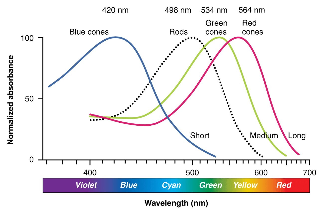
There are primarily two types of such cells: rod and cone cells. The rod cells are highly sensitive to photons insomuch that it can be triggered by even a single photon. These cells provide information about intensity of the light. On the other hand, cone cells are responsible for color perception. There are also three types of cones, each responding to different wavelengths, corresponding to the colors red, green, and blue. Thus, we usually refer to these colors as primary colors.
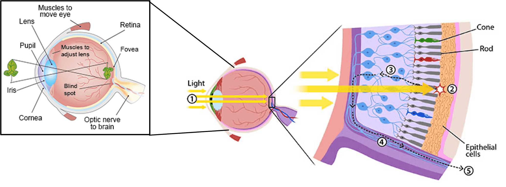
And in reality, color doesn’t have an inherent existence. Instead, our brain reconstructs color based on response levels from the three types of cone cells in our eyes. Human eyes can only response to a portion of the spectrum of those electromagnetic waves, commonly called visible light. Visible light refers to wavelengths in a range of 400 and 700 nm.
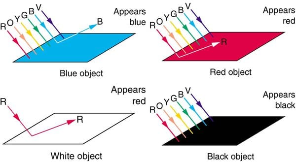
Then how the light interacts with materials? This process can be explained with quantum physics, but this post provides only a high-level overview of the process. When a material or an atom receives a photon, it enters an excited state. Subsequently, it returns to its normal state, releasing its energy into the surrounding space. This emission of energy contributes to various phenomena such as reflection, absorption, and transmission of light.
Therefore, realistic color representation in computer graphics requires quantifying light and materials, developing rules that describe their interaction, and presenting the results through some display medium so that the correct perceptions are created. Illumination models, also known as reflection models or shading models compute the colors of points on surfaces by considering local properties at the contact point of light and object surface.
Such reflection models have been used from the rasterization system (before ray tracing), while only some specific models such as specular reflection, diffusion reflection, and their combinations (Phone shading) have been used. And as we will see, BRDF is a general formulation that can represent all of these specific reflection models.
Surface Interaction: BxDF functions
The reflection models that we will discuss have been employed within rasterization systems, preceding the rendering equations, while only some specific models such as specular reflection, diffusion reflection, and their combinations (e.g. Phone model) have been used. And here, BRDF serves as a general formulation capable of representing all of these distinct reflection models.
In this section, we delve into alternative types of bi-directional distribution functions that are valuable in characterizing the interactions of light with surfaces.
BTDF
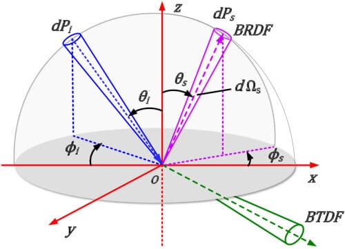
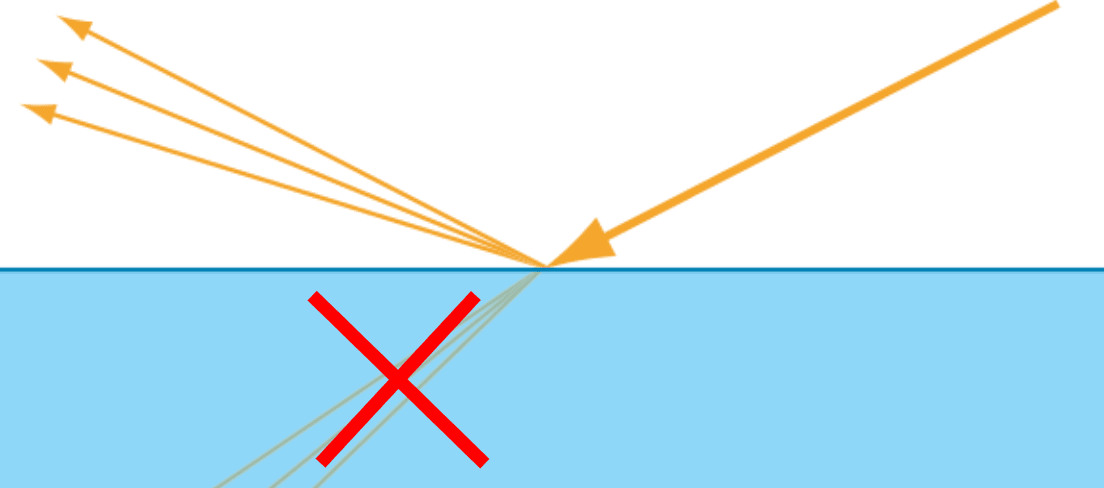
When light strikes the object surface, some of the light can be reflected, some of the light can be absorbed by the material, and some of the light can be transimitted, meaning it travels through a material completely. The bi-directional transmittance distribution function (BTDF) of a surface, denoted as $f_t (\mathrm{p}, \omega_{\mathrm{i}}, \omega_{\mathrm{t}})$ where $\omega_{\mathrm{i}}$ and $\omega_{\mathrm{r}}$ are lying in opposite hemispheres around the surface point $\mathrm{p}$, describes the distribution of transmitted light.
\[f_t\left(\mathrm{p}, \omega_{\mathrm{i}}, \omega_{\mathrm{t}}\right)=\frac{\mathrm{d} L_{\mathrm{t}}\left(\mathrm{p}, \omega_{\mathrm{t}}\right)}{\mathrm{d} E\left(\mathrm{p}, \omega_{\mathrm{i}}\right)}=\frac{\mathrm{d} L_{\mathrm{t}}\left(\mathrm{p}, \omega_{\mathrm{t}}\right)}{L_{\mathrm{i}}\left(\mathrm{p}, \omega_{\mathrm{i}}\right) \cos \theta_{\mathrm{i}} \mathrm{d} \omega_{\mathrm{i}}} \; \left[ \frac{1}{\textrm{sr}} \right]\]
BSDF
For ease of notation in equations, we typically denote the BRDF and BTDF when considered together as $f(\mathrm{p}, \omega_{\mathrm{i}}, \omega_{\mathrm{o}})$; we name this the bi-directional scattering distribution function (BSDF).
\[f\left(\mathrm{p}, \omega_{\mathrm{i}}, \omega_{\mathrm{o}}\right)=\frac{\mathrm{d} L_{\mathrm{o}}\left(\mathrm{p}, \omega_{\mathrm{o}}\right)}{\mathrm{d} E\left(\mathrm{p}, \omega_{\mathrm{i}}\right)}=\frac{\mathrm{d} L_{\mathrm{o}}\left(\mathrm{p}, \omega_{\mathrm{o}}\right)}{L_{\mathrm{i}}\left(\mathrm{p}, \omega_{\mathrm{i}}\right) \cos \theta_{\mathrm{i}} \mathrm{d} \omega_{\mathrm{i}}} \; \left[ \frac{1}{\textrm{sr}} \right]\]From the definition, we can integrate the differential of outgoing radiance over the sphere of incident directions around $\mathrm{p}$ to compute the outgoing radiance in direction $\omega_{\mathrm{o}}$:
\[L_{\mathrm{o}}\left(\mathrm{p}, \omega_{\mathrm{o}}\right) = \int_{S^2} f \left(\mathrm{p}, \omega_{\mathrm{i}}, \omega_{\mathrm{o}}\right) L_{\mathrm{i}} (\mathrm{p}, \omega_{\mathrm{i}}) \cos \theta_{\mathrm{i}} \; \mathrm{d}\omega_{\mathrm{i}}\]And this equation is often referred to as the scattering equation when the sphere $S^2$ is the domain as above, or the reflection equation when the integrated domain is constrained to the upper hemisphere $H^2$. It serves as a general mathematical function describing how light is scattered by a surface. However, in practice, it is typically separated into reflected (BRDF) and transmitted components (BTDF).
Indeed, the definition of the BSDF is not well standardized. For more information on its usage, please refer to this Wikipedia article.
BSSRDF
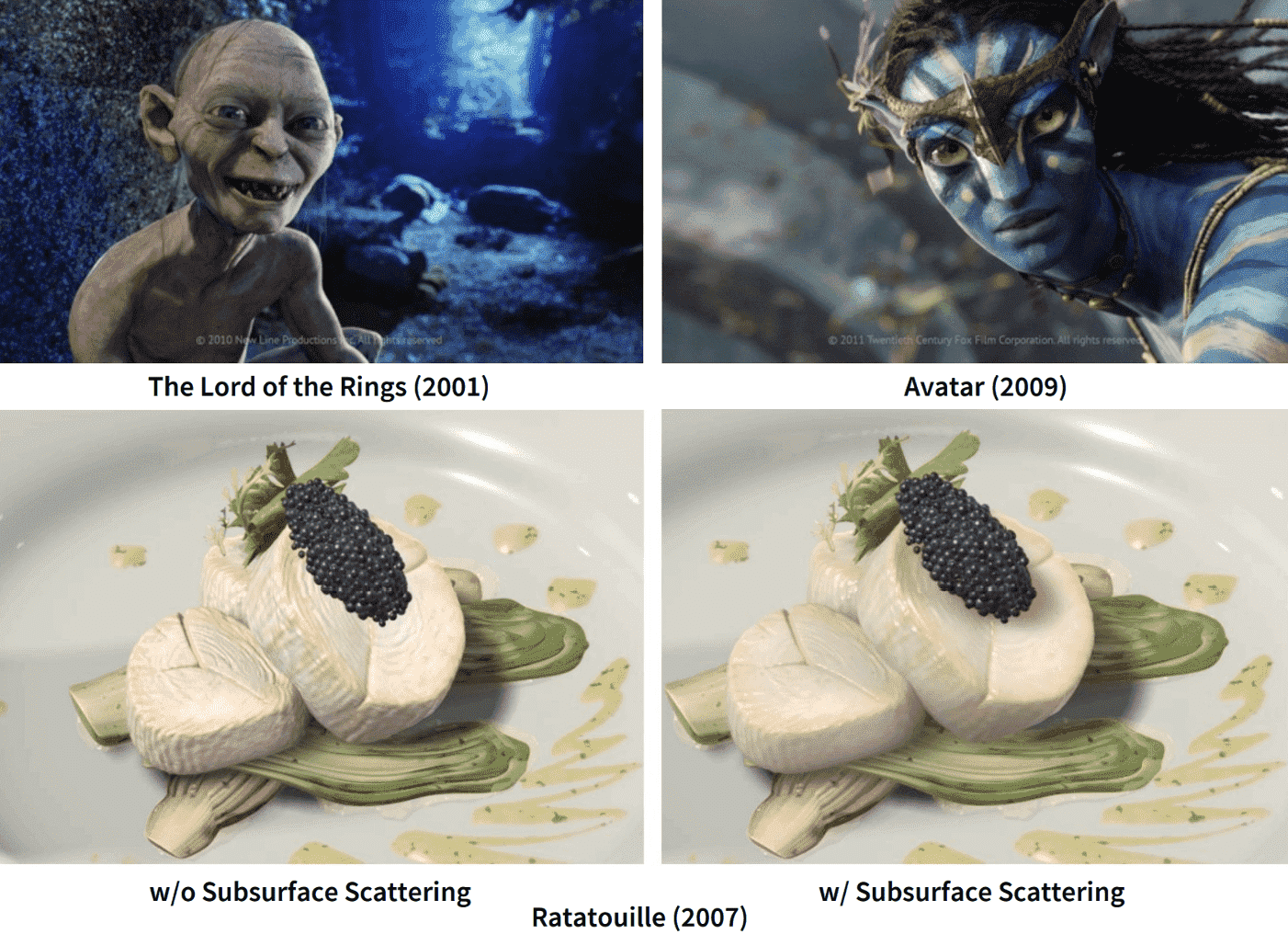
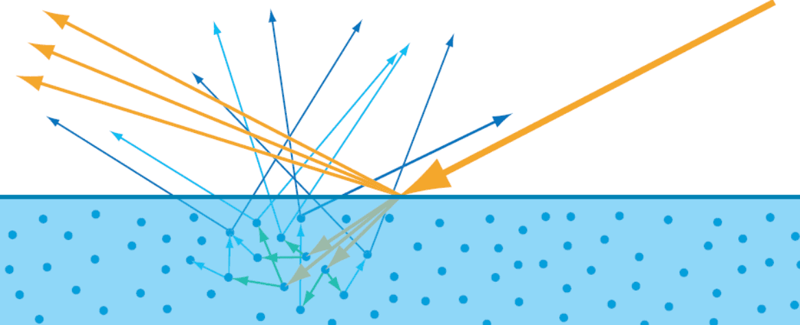
Reflection from translucent surfaces is more complex; a variety of materials ranging from skin and leaves to wax and liquids exhibit subsurface scattering, also known as subsurface light transport, where light that penetrates the surface at one point, gets scattered inside the material, and exits it at a different point.
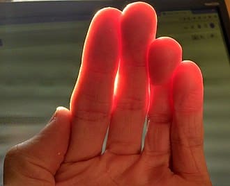
Suppose a ray of light contacts a surface at a point \(\mathrm{p}_{\mathrm{i}}\), and re-emitted from some point near \(\mathrm{p}_{\mathrm{i}}\), denote as \(\mathrm{p}_{\mathrm{o}}\), after multiple reflections in the material. This scattering can be formulated by bidirectional surface scattering reflectance distribution function (BSSRDF) \(S(\mathrm{p}_{\mathrm{i}}, \omega_{\mathrm{i}}, \mathrm{p}_{\mathrm{o}}, \omega_{\mathrm{o}})\).
The BSSRDF is defined as the ratio of exitant differential radiance at \(\mathrm{p}_{\mathrm{o}}\) in direction \(\omega_{\mathrm{o}}\) to the incident differential flux at \(\mathrm{p}_{\mathrm{i}}\) from direction \(\omega_{\mathrm{i}}\):
\[S(\mathrm{p}_{\mathrm{i}}, \omega_{\mathrm{i}}, \mathrm{p}_{\mathrm{o}}, \omega_{\mathrm{o}}) = \frac{\mathrm{d} L_{\mathrm{o}} (\mathrm{p}_{\mathrm{o}}, \omega_{\mathrm{o}})}{\mathrm{d} \Phi (\mathrm{p}_{\mathrm{i}}, \omega_{\mathrm{i}})}.\]

It is obvious that the BSSRDF necessitates the generalization of the scattering equation; 4D integration over surface area and incoming direction:
\[L_{\mathrm{o}}\left(\mathrm{p}_{\mathrm{o}}, \omega_{\mathrm{o}}\right)=\int_A \int_{\mathrm{H}^2(\mathbf{n})} S\left(\mathrm{p}_{\mathrm{o}}, \omega_{\mathrm{o}}, \mathrm{p}_{\mathrm{i}}, \omega_{\mathrm{i}}\right) L_{\mathrm{i}}\left(\mathrm{p}_{\mathrm{i}}, \omega_{\mathrm{i}}\right)\left|\cos \theta_{\mathrm{i}}\right| \mathrm{d} \omega_{\mathrm{i}} \mathrm{d} A .\]However, rendering materials using the BSSRDF can produce some spectacular results as shown in the following figure at the price of complexity of the rendering equation.
Types of Reflections
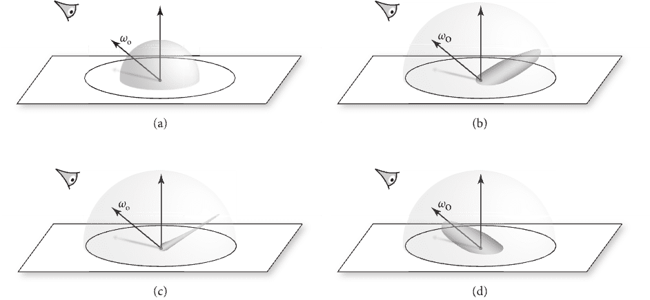
Before we start, to compare the resulting visual appearance, we can classify the types of reflection into the following 4 broad categories: ideal specular, non-ideal (glossy) specular, diffuse, retroreflective. Most real surfaces exhibit a mixture of these four behaviors.
-
Ideal Specular
- scatter incident light in a single outgoing direction;
- obeys reflection law;
- e.g. Mirror, glass;
-
Diffuse (Lambertian)
- an incident ray is reflected at many angles, rather than at just one angle;
- ideal diffuse surfaces, that scatter light equally in all directions, do not exist in the real world;
- obeys Lambert’s law;
- e.g. Matte;
-
Non-ideal Specular
- also known as glossy specular, or just specular
- scatter light preferentially in a set of reflected directions, thus directional diffuse and show blurry reflections of other objects;
- e.g. Plastic, High-gloss paint;
-
Retroreflective
- scatter light primarily back along the incident direction
- e.g., velvet, the Earth’s moon
Given a particular category of reflection, the reflectance distribution function may be isotropic or anisotropic.
-
Isotropic material
- if you choose a point on the surface and rotate it around its normal axis at that point, the distribution of light reflected at that point does not change;
- if $f_r ((\theta_{\mathrm{i}}, \phi_{\mathrm{i}}) \to (\theta_{\mathrm{r}}, \phi_{\mathrm{r}}))$ can be reduced into a function with 3 parameters $f_r (\theta_{\mathrm{i}}, \theta_{\mathrm{r}}, \phi_{\mathrm{i}} - \phi_{\mathrm{r}})$
-
Anisotropic material
- reflect different amounts of light as you rotate them around its normal axis at the given point;
- e.g., hair, cloth, etc.
Classes of Materials
Light comprises electromagnetic waves, thereby establishing a close correlation between the optical characteristics of a substance and its electrical properties. Materials are typically categorized into three primary optical classes: metal (or conductor), dielectric (or insulator; while not precisely synonymous, they are often treated interchangeably in graphics), and semiconductor. However, given that visible object surfaces seldom exhibit semiconductor properties, for pragmatic considerations, we can adopt a simplified grouping into metals and non-metals.
- Dielectrics
Materials (typically, non-metals) that don't conduct electricity. They have real-valued refraction indices and transmit a portion of the incident illumination.- Examples: Plastic, Stone, Wood, Leather, Glass, Water, Air
$\mathbf{Fig\ 9.}$ Non-metals (SIGGRAPH) - Conductors
In conductors, valence electrons can freely traverse within the their atomic lattice, allowing electric currents to flow from one place to another. This fundamental atomic property translates into a profoundly different behavior when a conductor is subjected to electromagnetic radiation such as visible light: the material exhibits opaque and reflects back a substantial portion of the incident illumination.
These materials have the distincitve property of absorbing all of refracted light. While a fraction of the incoming light also penetrates into the interior of the conductor, it is rapidly absorbed, and total absorption typically occurs within the top $0.1\textrm{nm}$ of the material. Therefore, only exceedingly thin metal films can transmit appreciable quantities of light. In contrast to dielectrics, conductors theoretically have a complex-valued refraction index $\bar{\eta} = \eta + k \mathrm{i}$- Examples: Metals
$\mathbf{Fig\ 10.}$ Metals (SIGGRAPH)
Dielectrics, conductors, and semiconductors are all governed by the same Fresnel equations that are introduced in the next section.
Basic Reflection and Refraction
Ideal Diffuse Relection
An ideal diffuse surface scatters incident illumination equally in all directions. (Although this reflection model is not physically plausible, it is a reasonable approximation to many real-world surfaces such as matte paint.) Mathematically, this means
\[f_r (\omega_{\mathrm{i}}, \omega_{\mathrm{r}}) = \frac{\rho}{\pi}\]where $\rho$ is albedo; the ratio between outgoing irradiance and incoming irradiance. This originate from the following equation:
\[\begin{aligned} L_\mathrm{o} & = \int_{H^2} f_r (\omega_{\mathrm{i}}, \omega_{\mathrm{r}}) L_{\mathrm{i}} (\omega_{\mathrm{i}}) \cos \theta_{\mathrm{i}} \; d \omega_{\mathrm{i}} \\ & = \frac{\rho}{\pi} \int_{H^2} L_{\mathrm{i}} (\omega_{\mathrm{i}}) \cos \theta_{\mathrm{i}} \; d \omega_{\mathrm{i}} = \frac{\rho}{\pi} E_{\mathrm{i}} \\ E_\mathrm{o} & = \int_{H^2} L_{\mathrm{o}} \cos \theta \; \mathrm{d}\omega = \frac{\rho}{\pi} E_{\mathrm{i}} \int_{H^2} \cos \theta \; \mathrm{d}\omega = \rho E_{\mathrm{i}} \end{aligned} \\ \therefore \rho = \frac{E_{\mathrm{o}}}{E_{\mathrm{i}}} \leq 1\]Ideal Specular Reflection and Refraction
Ideal specular surfaces only reflect or refract light in a singular direction, dictated by the principles of the reflection law and Snell’s law. And the Fresnel equations delineate the propotion of incident light reflected from a surface; thus provides the fraction of incoming light that is reflected or transmitted.
Reflection
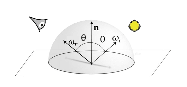
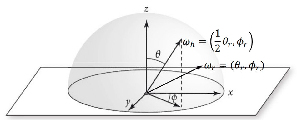
In an ideal specular reflection, the incident light is simply reflected across the normal. Given the direction of the incident light $\omega_{\mathrm{i}} = (\theta_{\mathrm{i}}, \phi_{\mathrm{i}})$, the law of reflection provides the resulting outgoing direction $\omega_{\mathrm{r}} = (\theta_{\mathrm{r}}, \phi_{\mathrm{r}})$ of the given incident light:
Given incident light from a direction $(\theta_{\mathrm{i}}, \phi_{\mathrm{i}})$, the single reflected direction $(\theta_{\mathrm{r}}, \phi_{\mathrm{r}})$ following an interaction with an ideal specular surface is simply given by $$ (\theta_{\mathrm{r}}, \phi_{\mathrm{r}}) = (\theta_{\mathrm{i}}, \phi_{\mathrm{i}} + \pi) $$ With the direction vector representation, with the normal vector $\mathbf{n}$ at the contact point, the following relation is satisfied: $$ \omega_{\mathrm{r}} = - \omega_{\mathrm{i}} + 2 (\omega_{\mathrm{i}} \cdot \mathbf{n}) \mathbf{n}. $$
$\mathbf{Proof.}$
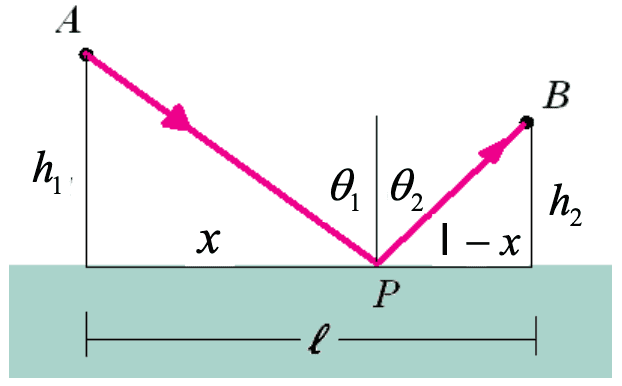
This proof is borrowed from Giancoli et al. 2013. The law of reflection can be derived using Fermat’s principle, which states that light will follow the path that requires the least amount of time, as compared to other nearby paths, to pass between two points.
Consider the light ray shown in the figure below. A ray starting at point $\mathrm{A}$ reflects off the surface at point $\mathrm{P}$ before arriving at point $\mathrm{B}$, a horizontal distance $\ell$ from point $\mathrm{A}$. We calculate the length of each path and divide the length by the speed of light to determine the time required for the light to travel between the two points. Then we obtain
\[t = \frac{\sqrt{x^2 + h_1^2}}{c} + \frac{\sqrt{(\ell - x)^2 + h_2^2}}{c}\]
To minimize the time,
\[0 = \frac{\mathrm{d}t}{\mathrm{d}x} = \frac{x}{c \sqrt{x^2 + h_1^2}} + \frac{- (\ell - x)}{c \sqrt{(\ell - x)^2 + h_2^2}}\]which is equivalent to
\[\frac{x}{\sqrt{x^2 + h_1^2}} = \frac{(\ell - x)}{\sqrt{(\ell - x)^2 + h_2^2}}\]Thus it suggests $\sin \theta_{1} = \sin \theta_{2}$, which proves the angular form of the reflection law.
And with this result, we can derive the vector form of reflection law. The direction vector $\omega$ lying in a plane can be decomposed into a sum of two components: $\omega_{\Vert}$ parallel to the normal $\mathbf{n}$, and $\omega_{\perp}$ perpendicular to the normal:
\[\begin{aligned} \omega_{\Vert} & = \cos \theta \cdot \mathbf{n} = (\mathbf{n} \cdot \omega) \mathbf{n} \\ \omega_{\perp} & = \omega - \omega_{\Vert} = \omega - (\mathbf{n} \cdot \omega) \mathbf{n} \end{aligned}\]Then the reflected direction $\omega_{\mathrm{r}}$ with respect to the incident direction $\omega_{\mathrm{i}}$, we have
\[\begin{aligned} \omega_{\mathrm{r}}=\omega_{\mathrm{r} \perp}+\omega_{\mathrm{r} \|} & =-\omega_{\mathrm{i} \perp}+\omega_{\mathrm{i} \|} \\ & =-\left(\omega_{\mathrm{i}}-\left(\mathbf{n} \cdot \omega_{\mathrm{i}}\right) \mathbf{n}\right)+\left(\mathbf{n} \cdot \omega_{\mathrm{i}}\right) \mathbf{n} \\ & =-\omega_{\mathrm{i}}+2\left(\mathbf{n} \cdot \omega_{\mathrm{i}}\right) \mathbf{n} . \end{aligned}\] \[\tag*{$\blacksquare$}\]Intuitively, we want the specular reflection BRDF to be zero everywhere except at the reflection direction. Initially, one might consider using delta functions to confine the incident direction to the specular reflection direction $\omega_{\mathrm{r}}$. This intuition naturally suggests the following proportionality of BRDF:
\[f_r (\omega_{\mathrm{i}}, \omega_{\mathrm{r}}) \propto \delta (\omega_{\mathrm{i}} - R(\omega_{\mathrm{o}}, \mathbf{n}))\]where $R(\omega, \mathbf{n}) = -\omega+2\left(\mathbf{n} \cdot \omega\right) \mathbf{n}$, thus $R(\omega_{\mathrm{o}}, \mathbf{n}) = \omega_{\mathrm{i}}$ if $\omega_{\mathrm{o}} = -\omega_{\mathrm{i}}+2\left(\mathbf{n} \cdot \omega_{\mathrm{i}}\right) \mathbf{n}$ and we can write $f_r$ as follows:
\[f_r (\omega_{\mathrm{i}}, \omega_{\mathrm{r}}) = \delta (\omega_{\mathrm{i}} - \omega_{\mathrm{r}}) F_r (\omega_{\mathrm{i}}).\]Plugging it into the reflection equation:
\[L_{\mathrm{o}} = \int f_r (\omega_{\mathrm{i}}, \omega_{\mathrm{r}}) L_{\mathrm{i}} (\omega_{\mathrm{i}}) \cos \theta_{\mathrm{i}} \; \mathrm{d}\omega_{\mathrm{i}}\]we obtain $L_{\mathrm{o}} (\omega_{\mathrm{o}}) = F_{\mathrm{r}} (\omega_{\mathrm{r}}) L_{\mathrm{i}} (\omega_{\mathrm{r}}) \cos \theta_{\mathrm{r}}$, involving the extra factor of $\cos \theta_{\mathrm{r}} = \cos \theta_{\mathrm{i}}$. Consequently, we divide out this factor for the ideal specular BRDF:
\[f_r (\omega_{\mathrm{i}}, \omega_{\mathrm{r}}) = \frac{\delta (\omega_{\mathrm{i}} - \omega_{\mathrm{r}}) F_r (\omega_{\mathrm{i}})}{\cos \theta_{\mathrm{i}}}.\]Refraction
Similarly with reflection, ideal specular surfaces only refract light in one specific direction. And its direction is determined by Snell’s law, which involves the refraction index $\eta$ that describes how much more slowly light travels in a particular medium than in a vacuum, for the medium the incident ray is in and it is entering.
If the incident light with direction $\omega_{\mathrm{i}} = (\theta_{\mathrm{i}}, \phi_{\mathrm{o}})$ about the surface normal and it refracts into a single transmitted direction $\omega_{\mathrm{t}} = (\theta_{\mathrm{t}}, \phi_{\mathrm{t}})$ located on the opposite side of the interface, tbe following equation is satisfied: $$ \eta_{\mathrm{i}} \sin \theta_{\mathrm{i}} = \eta_{\mathrm{t}} \sin \theta_{\mathrm{t}} \quad \text{ and } \quad \phi_{\mathrm{t}} = \phi_{\mathrm{i}} + \pi. $$ For the direction vector representation, with the normal vector $\mathbf{n}$ at the contact point and relative index of refraction $\eta = \eta_{\mathrm{t}} / \eta_{\mathrm{i}}$, the following relation is satisfied: $$ \omega_{\mathrm{t}} = - \frac{\omega_{\mathrm{i}}}{\eta} + \left[ \frac{\omega_{\mathrm{i}} \cdot \mathbf{n} }{\eta} - \cos \theta_{\mathrm{t}} \right] \mathbf{n} $$

$\mathbf{Proof.}$
This proof is borrowed from Giancoli et al. 2013. The law of reflection can be derived using Fermat’s principle, which states that light will follow the path that requires the least amount of time, as compared to other nearby paths, to pass between two points.
Consider the light ray shown in the figure below. A ray starting at point $\mathrm{A}$ travels to point $\mathrm{B}$, a horizontal distance $\ell$ from point $\mathrm{A}$, entering the meidum with different indices of refraction at point $\mathrm{P}$. We calculate the length of each path and divide the length by the speed of light to determine the time required for the light to travel between the two points. Then we obtain
\[t = \frac{\sqrt{x^2 + h_1^2}}{c / n_1} + \frac{\sqrt{(\ell - x)^2 + h_2^2}}{c / n_2}\]
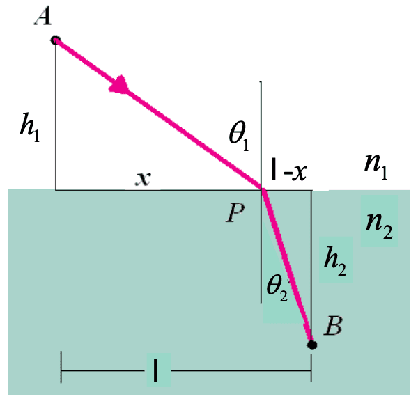
To minimize the time,
\[0 = \frac{\mathrm{d}t}{\mathrm{d}x} = \frac{n_1 x}{c \sqrt{x^2 + h_1^2}} + \frac{- n_2 (\ell - x)}{c \sqrt{(\ell - x)^2 + h_2^2}}\]which is equivalent to
\[\frac{n_1 x}{\sqrt{x^2 + h_1^2}} = \frac{n_2 (\ell - x)}{\sqrt{(\ell - x)^2 + h_2^2}}\]Thus it suggests $n_1 \sin \theta_{1} = n_2 \sin \theta_{2}$, which proves the angular form of the Snell’s law.
And ith this result, we can derive the vectorial form of Snell’s law. The direction vector $\omega$ lying in a plane can be decomposed into a sum of two components: $\omega_{\Vert}$ parallel to the normal $\mathbf{n}$, and $\omega_{\perp}$ perpendicular to the normal. Then, from the angular form, for the relative index of refraction $\eta = \eta_{\mathrm{t}} / \eta_{\mathrm{i}}$ we have
\[\omega_{\mathrm{t} \perp} = - \frac{\omega_{\mathrm{i} \perp}}{\eta}\]Equivalently, since $\omega_{\perp} = \omega - \omega_{\Vert}$,
\[\omega_{\mathrm{t} \perp} = - \frac{-\omega_{\mathrm{i}} + (\omega_{\mathrm{i}} \cdot \mathbf{n}) \mathbf{n}}{\eta}\]The parallel component points into the direction $-\mathbf{n}$, and its magnitude is given by $\cos \theta_{\mathrm{t}}$. That is,
\[\omega_{\mathrm{t} \Vert} = - \cos \theta_{\mathrm{t}} \mathbf{n}\]Putting all the above together,
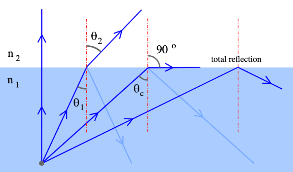
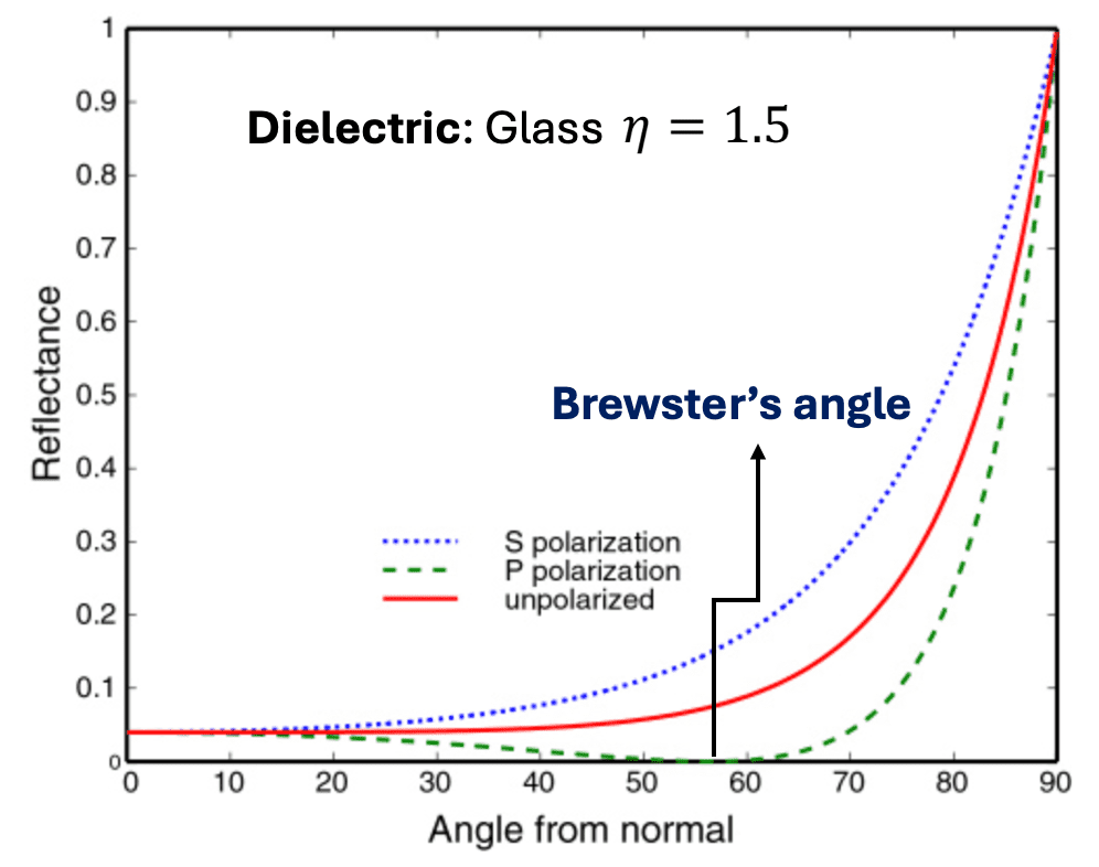
\[\begin{aligned} \omega_{\mathrm{t}} & = \omega_{\mathrm{t} \perp} + \omega_{\mathrm{t} \Vert} \\ & = - \frac{\omega_{\mathrm{i}}}{\eta} + \left[ \frac{\omega_{\mathrm{i}} \cdot \mathbf{n} }{\eta} - \cos \theta_{\mathrm{t}} \right] \mathbf{n}. \end{aligned}\] \[\tag*{$\blacksquare$}\]When light transitions into a less optically dense medium, i.e. $\eta_{\mathrm{t}} < \eta_{\mathrm{i}}$, the interface turns into an ideal reflector at certain angles so that no light is transmitted. In other words, light approaching the interface (boundary) from one medium to another are not refracted but instead completely reflected back into the initial medium. This phenomenon is called total internal reflection, occuring when the incident angle $\theta_{\mathrm{i}}$ is greater than the critical angle (also called Brewster’s angle) $\theta_{\mathrm{c}}$: $$ \theta_{\mathrm{i}} > \theta_{\mathrm{c}} = \sin^{-1} (1 / \eta) = \sin^{-1} (\eta_{\mathrm{t}} / \eta_{\mathrm{i}}) $$
With the result of Snell’s law, we are now possible to derive the BTDF for (ideal) specular transmission. Denote the fraction of indcident energy that is transmitted to the outgoing direction by $\tau = 1 - F_{\mathrm{r}} (\omega_{\mathrm{i}})$. That is, $\mathrm{d} \Phi_{\mathrm{t}} = \tau \mathrm{d} \Phi_{\mathrm{i}}$. By definition of radiance, we obtain
\[L_{\mathrm{t}} \cos \theta_{\mathrm{t}} \; \mathrm{d}A \; \mathrm{d}\omega_{\mathrm{t}} = \tau L_{\mathrm{i}} \cos \theta_{\mathrm{i}} \; \mathrm{d}A \; \mathrm{d}\omega_{\mathrm{i}}\]or equivalently
\[L_{\mathrm{t}} \cos \theta_{\mathrm{t}} \; \mathrm{d}A \; \sin \theta_{\mathrm{t}} \; d\theta_{\mathrm{t}} \mathrm{d}\phi_{\mathrm{t}} = \tau L_{\mathrm{i}} \cos \theta_{\mathrm{i}} \; \mathrm{d}A \; \sin \theta_{\mathrm{i}} \; d\theta_{\mathrm{i}} \mathrm{d}\phi_{\mathrm{i}}\]Note that we have $\eta_{\mathrm{t}} \cos \theta_{\mathrm{t}} \; \mathrm{d} \theta_{\mathrm{t}} = \eta_{\mathrm{i}} \cos \theta_{\mathrm{i}} \; \mathrm{d} \theta_{\mathrm{i}}$ by differentiating the Snell’s law. Furthermore, $\phi_{\mathrm{i}} = \phi_{\mathrm{t}} + \pi$, therefore $\mathrm{d}\phi_{\mathrm{i}} = \mathrm{d}\phi_{\mathrm{t}}$. These relations then simplify the equation as follows:
\[L_\mathrm{t} = \tau L_\mathrm{i} \frac{\eta_{\mathrm{t}}^2}{\eta_{\mathrm{i}}^2}\]Similar with the BRDF for specular reflection, we should divide out $\cos \theta_{\mathrm{i}}$ term to get the right BTDF for specular transmission:
\[f_{\mathrm{t}} (\omega_{\mathrm{t}}, \omega_{\mathrm{i}}) = \frac{\eta_{\mathrm{t}}^2}{\eta_{\mathrm{i}}^2} (1 - F_{\mathrm{r}} (\omega_{\mathrm{i}})) \frac{\delta (\omega_{\mathrm{i}} - T (\omega_{\mathrm{t}}, \mathbf{n}))}{\cos \theta_{\mathrm{i}}}\]where $T (\omega_{\mathrm{i}}, \mathbf{n}) = - \frac{\omega_{\mathrm{i}}}{\eta} + \left[ \frac{\omega_{\mathrm{i}} \cdot \mathbf{n} }{\eta} - \cos \theta_{\mathrm{t}} \right] \mathbf{n}$. That is, if $\omega_{\mathrm{t}}$ is the vector that results from the transmission of the incident vector $\omega_{\mathrm{i}}$ at the same interface with surface normal $\mathbf{n}$, i.e. $\omega_{\mathrm{t}} = T (\omega_{\mathrm{i}}, \mathbf{n})$, then $T (\omega_{\mathrm{t}}, \mathbf{n}) = \omega_{\mathrm{i}}$.
Fresnel Equations
In addition to the reflected and transmitted directions, it is also necessary to compute the fraction of incoming light that is reflected or transmitted. For physically accurate reflection or refraction, these terms are directionally dependent and cannot be captured by constant per-surface scaling amounts. Fresnel derived a set of equations called the Fresnel equations that describe the amount of light energy that is reflected and refracted from perfectly specular surfaces.
While we employed geometric optics to characterize light, it is essential to acknowledge that light fundamentally constitutes an electromagnetic wave, with its electric field oscillating perpendicular to the direction of propagation. And light is called unpolarized when the orientation of this electric field fluctuates randomly over time. Numerous prevalent light sources, including sunlight, LED spotlights, and incandescent bulbs, emit unpolarized light. Conversely, when the orientation of light’s electric field is precisely defined, it is termed polarized light. The primary source of polarized light commonly encountered is a laser. In case of polarized lights, we can classify them into three types of polarizations depending on how the orientation of electric field:
-
Linear polarization
confined to a single plane along the direction of propagation -
Circular polarization
consists of two linear components perpendicular to each other, equal in amplitude, but have phase difference of $\pi/2$ -
Elliptical polarization
the combination of two linear components with different amplitudes and/or a phase difference that is not $\pi/2$.
And the two orthogonal linear polarization states that are most important for reflection and transmission are referred to as S- and P-polarization.
- P-polarized: polarized parallel to the plane of incidence
- S-polarized: polarized perpendicular to the plane of incidence
The Fresnel equations relate the amplitudes of the reflected wave $E_{\mathrm{r}}$ given an incident wave with a known amplitude $E_{\mathrm{i}}$. For S- and P-polarized lights, the ratio of these amplitudes is given by
\[\begin{aligned} & r_s= \frac{E_{\mathrm{r}}^s}{E_{\mathrm{i}}^s} = \left|\frac{\eta_t \cos \theta_i-\eta_i \cos \theta_t}{\eta_t \cos \theta_i + \eta_i \cos \theta_t}\right| \\ & r_p= \frac{E_{\mathrm{r}}^p}{E_{\mathrm{i}}^p} = \left|\frac{\eta_i \cos \theta_i-\eta_t \cos \theta_t}{\eta_i \cos \theta_i + \eta_t \cos \theta_t}\right| \end{aligned}\]
For the proof of Fresnel equations, please refer to the lecture note of Matthew Schwartz. However, since we are assuming geometric optics, we focus on the overall power carried by the wave, which is given by the square of the amplitude rather than amplitude itself. Integrating these equations with the assumption of unpolarized light in geometric optics leads to the Fresnel reflectance $F_{\mathrm{r}}$ that indicates the proportion of reflection:
\[F_{\mathrm{r}} = \frac{1}{2} (r_s^2 + r_p^2)\]And by the energy conservation assumption, the proportion of refraction is then computed by $T_\mathrm{r} = 1 - F_{\mathrm{r}}$.
As an example, the following figure illustrates the reflectance for a typical dielectric materials, especially when the light proceeds to the glass ($\eta = 1.5$) from the vacuum. Most glasses and plastics exhibit refractive indices approximately at $1.5$, resulting in a reflectance of merely 4% under normal incidence, yet escalating to 100% at grazing angles. This phenomenon is the reason why it’s hard to groom your hair in front of a shop window, because you are looking at the angle of minimum reflectance.
Schlick Approximation
The Fresnel equations are exact, but complicated to evaluate. In computer graphics, the most commonly used approximation for the Fresnel effect is Schlick’s approximation:
\[F_\mathrm{r} (\omega_{\mathrm{i}}) \approx F_0 + (1 - F_0) \times ( 1 - (\mathbf{n} \cdot \omega_\mathrm{i}))^5\]where $\mathbf{n}$ is the normal vector of the reflection and
\[F_0 = \frac{(\eta_{i} - \eta_{t})^2}{(\eta_{i}+\eta_{t})^2}\]With considerably simpler and more affordable computation, the Schlick approximation can achieve a speedup of 32 times with less than 1% average error (in optimized implementation).
Fresnel-Modulated Specular Reflection and Transmission
Utilizing the Fresnel equation that provides the fraction of transmitted light, one can practically simulate the (ideal) specular reflection and transmission simultaneously. By integrating the ideal specular BSDF into the scattering equation:
\[\begin{aligned} & L_{\mathrm{o}}\left(\mathrm{p}, \omega_{\mathrm{o}}\right)=\int_{H^2} f \left(\mathrm{p}, \omega_{\mathrm{i}} \rightarrow \omega_{\mathrm{o}}\right) L_{\mathrm{i}}\left(\mathrm{p}, \omega_{\mathrm{i}}\right) \cos \theta_{\mathrm{i}} \mathrm{~d} \omega_{\mathrm{i}} \\ & =\int_{H^2}\left(F_{\mathrm{r}} \frac{\delta\left(\omega_{\mathrm{i}}-R\left(\omega_{\mathrm{o}}, \mathbf{n}\right)\right)}{\cos \theta_{\mathrm{i}}}+\left(1-F_{\mathrm{r}}\right) \frac{\delta\left(\omega_{\mathrm{i}}-T\left(\omega_{\mathrm{o}}, \mathbf{n}\right)\right)}{\cos \theta_{\mathrm{i}}}\right) L_{\mathrm{i}}\left(\mathrm{p}, \omega_{\mathrm{i}}\right) \cos \theta_{\mathrm{i}} \mathrm{~d} \omega_{\mathrm{i}} \\ & =F_{\mathrm{r}} \int_{H^2} \frac{\delta\left(\omega_{\mathrm{i}}-R\left(\omega_{\mathrm{o}}, \mathbf{n}\right)\right)}{\cos \theta_{\mathrm{i}}} L_{\mathrm{i}}\left(\mathrm{p}, \omega_{\mathrm{i}}\right) \cos \theta_{\mathrm{i}} \mathrm{~d} \omega_{\mathrm{i}}+\left(1-F_{\mathrm{r}} \right) \int_{H^2} \frac{\delta\left(\omega_{\mathrm{i}}-T\left(\omega_{\mathrm{o}}, \mathbf{n}\right)\right)}{\cos \theta_{\mathrm{i}}} L_{\mathrm{i}}\left(\mathrm{p}, \omega_{\mathrm{i}}\right) \cos \theta_{\mathrm{i}} \mathrm{~d} \omega_{\mathrm{i}} \\ & =F_{\mathrm{r}} L_{\mathrm{i}}\left(R\left(\omega_{\mathrm{o}}, \mathbf{n}\right)\right)+\left(1-F_{\mathrm{r}} \right) L_{\mathrm{i}}\left(T\left(\omega_{\mathrm{o}}, \mathbf{n}\right)\right) \end{aligned}\]where $R\left(\omega_{\mathrm{o}}, \mathbf{n}\right)$ and $T\left(\omega_{\mathrm{o}}, \mathbf{n}\right)$ are the vector generated by the reflection and refraction of $\omega_{\mathrm{o}}$ at the interface with surface normal $\mathbf{n}$, respectively.
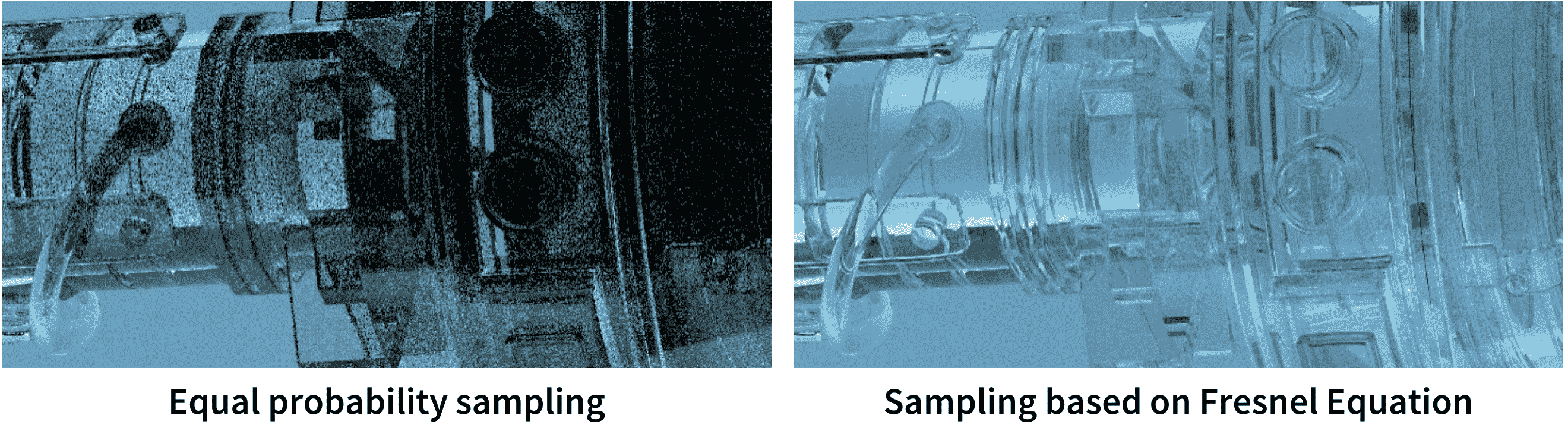
Note that each ray hit the surface causes two rays, one for reflection and another for transmission, the number of rays grow exponentially for each bounce in ray tracing framework. To enhance the efficiency, we can construct the following Monte-Carlo Estimator that selects one of the ray in each bounce:
\[L_{\mathrm{o}} (\mathrm{p}, \omega_{\mathrm{o}}) \approx \begin{cases} L_{\mathrm{i}} (R (\omega_{\mathrm{o}}, \mathbf{n})) & \quad \text{ if } \xi < F_{\mathrm{r}} \\ L_{\mathrm{i}} (T (\omega_{\mathrm{o}}, \mathbf{n})) & \quad \text{ otherwise } \\ \end{cases}\]$\mathbf{Fig\ 18}$ shows the benefit of sampling in this way compared to an equal split between reflection and transmission.
Empirical Illumination Models
Broadly, the illumination model is segmented into two distinct branches: empirical models, which offer simplified approximations of observed phenomena and do not have no physical basis, and physically-based models, which intricately model the genuine physics underlying light interactions. While physically-based models facilitate the attainment of photorealistic renderings, the initial illumination models were primarily empirical in nature. Hence, in chronological progression, we first delve into the realm of empirical models.
Lambert’s model
The simplest model is Lambert’s model for idealized diffuse materials. In this model, the BRDF is a constant as described earlier:
\[f_r (\mathrm{p}, \omega_\mathrm{i}, \omega_{\mathrm{o}}) = \frac{\rho_d}{\pi} := K_d\]where $\rho_d$ is the albedo of the material.
Phong model
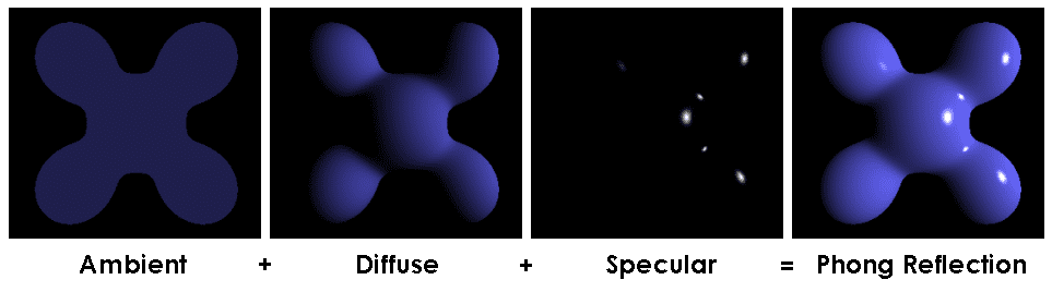
The most popular but simplest empirical model is the Phong illumination model. It formulates the reflection of light on the surface by the linear combination of the (ideal) diffuse reflection, which simulates the directional impact, with the (glossy) specular refection that simulates the bright spot on the shiny objects. The BRDF of the Phong model is given by
\[f_r (\mathrm{p}, \omega_\mathrm{i}, \omega_{\mathrm{r}}) = K_d + K_s \frac{(R(\omega_{\mathrm{i}}, \mathbf{n}) \cdot \omega_{\mathrm{r}})^\alpha}{\mathbf{n} \cdot \omega_{\mathrm{i}}}\]where $R\left(\omega_{\mathrm{i}}, \mathbf{n}\right)$ is the vector generated by the reflection of $\omega_{\mathrm{i}}$ at the interface with surface normal $\mathbf{n}$. It’s worth noting that the Phong model predates the Kajiya’s invention of the rendering equation by over a decade. To maintain consistency with this historical precedence, we divided the specular term by $\cos \theta_{\mathrm{i}} = \mathbf{n} \cdot \omega_{\mathrm{i}}$ and adopt the assumption of a one-directional point light source emanating from $\omega_{\mathrm{i}}$ in the reflection equation, i.e. $L_{\mathrm{i}}(\omega) = L \delta(\omega_{\mathrm{i}} - \omega)$. Consequently, the reflected radiance is derived as
\[L_{\mathrm{r}} (\mathrm{p}, \omega_{\mathrm{r}}) = \left[ K_d (\omega_{\mathrm{i}} \cdot \mathbf{n}) + K_s (R(\omega_{\mathrm{i}}, \mathbf{n}) \cdot \omega_{\mathrm{r}})^\alpha \right] \times L_{\mathrm{i}} (\mathrm{p}, \omega_{\mathrm{i}})\]where the following parameters are defined for each material:
- $K_s$: specular reflection constant, the ratio of reflection of the specular term of incoming light
- $K_d$: diffuse reflection constant, Lambertian reflectance
- $\alpha > 0$: shininess, larger for surfaces that are smoother and more mirror-like.
Since leaving $\cos \theta_{\mathrm{i}}$ out from the rendering equation is physically nonsense, some literatures remove the denominator and write
\[f_r (\mathrm{p}, \omega_\mathrm{i}, \omega_{\mathrm{r}}) = K_d + K_s (R(\omega_{\mathrm{i}}, \mathbf{n}) \cdot \omega_{\mathrm{r}})^\alpha\]
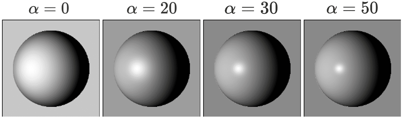
This model is distinguished by its modeling of the specular component, which is based on the Phong’s informal observation. Phong noted that glossy (shiny) surfaces exhibit focused highlights that diminish rapidly, whereas matte surfaces feature diffuse highlights that fade gradually. Consequently, Phong designed the specular lobe as a $\alpha$-th power of the cosine of the angle between the outgoing direction and the ideal reflection direction, of which exponential $\alpha$, called shininess is vary materials.
\[f_{\text{specular}} (\omega_{\mathrm{i}}, \omega_{\mathrm{r}}) \propto \cos^\alpha \theta_{\mathrm{r}} = \left( R(\omega_{\mathrm{i}}, \mathbf{n}) \cdot \omega_{\mathrm{r}} \right)^\alpha\]
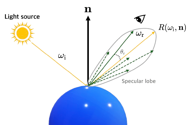
Note that $\alpha$ controls how quickly the highlight falls off. It is larger for glossy surfaces and smaller for matt surfaces. And for $\alpha = \infty$, it represents reflection of ideal reflectors.
Consequently, the regions of the scene not directly illuminated are not visible, as we soley account for the reflection term without incorporating the indirect light modeling. In Phong model, therefore, the absence of indirect lighting is approximated by a constant radiance $L_{\mathrm{e}} (\omega_{\mathrm{o}}) = K_a$, representing the radiance that ambient light would yield on an ideal white surface. Given that the Phong model is non-physical in nature, users can freely adjust the parameters $K_a$, $K_d$, $K_s$ and the exponent $\alpha$.
Blinn-Phong model
In particular circumstances, notably when $\theta_{\mathrm{r}} > 90^\circ$ with low shininess materials, leading to an expansive (rough) specular area, the specular reflections may deteriorate. One might misinterpret that no light should be received at angles exceeding 90 degrees, however if a material with a low specular exponent is utilized, the specular radius can be extensive enough to yield contributions beyond $\theta_{\mathrm{r}} > 90^\circ$.
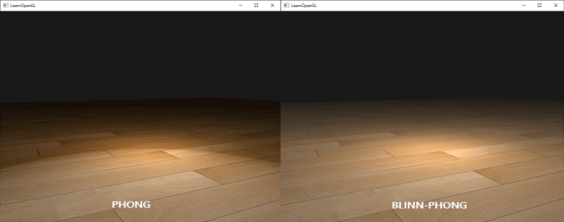
This issue can be mitigated by simply changing the computation. James F. Blinn introduced another a modification, called halfway vector for computing Phong reflection, as referenced in the work of Ken Torrance. This vector is motivated by microfacet models we’ll discuss, hence we’ll omit those details just for now.
\[\mathbf{h} = \frac{ \omega_{\mathrm{i}} + \omega_{\mathrm{r}} }{\lVert \omega_{\mathrm{i}} + \omega_{\mathrm{r}} \rVert}\]
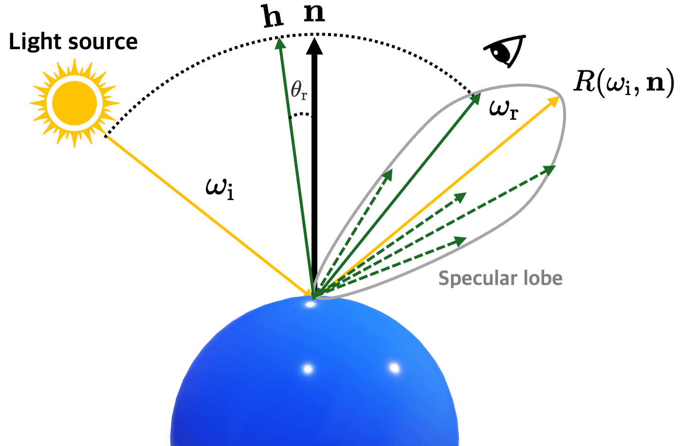
and the specular term compares the half-way vector to the surface normal, rather than comparing the reflection vector to the view direction:
\[\textrm{specular term} \propto K_s (\mathbf{h} \cdot \mathbf{n})^\alpha\]Note that the angle between the half-way vector and the surface normal is always less than 90 degrees. This modified model is called the Blinn-Phong reflection model or just the Blinn reflection model. This model exhibits better efficiency compared to the Phong model as it circumvents the calculation of the reflected direction $R(\omega_{\mathrm{i}}, \mathbf{n})$.
Modified Blinn-Phong model
While the simplicity of the Phong model is appealing, it has another severe limitation that the (Blinn-) Phong BRDF is not guaranteed to energy conserving. While this isn’t a significant concern for local illumination, it does pose challenges for global lighting simulations where physical accuracy is paramount.
To guarantee the energy conservation with $\rho_d + \rho_s \leq 1$ (sufficent, but not necessary conditions for conservation), we can multiply some normalization factors as follows.
For the Phong BRDF, without cosine term in the denominator of the specular term: $$ f_{r, \textrm{Phong}} (\omega_{\mathrm{i}}, \omega_{\mathrm{r}}) = \frac{K_d}{\pi} + \frac{\alpha + 2}{2\pi} K_s (R(\omega_{\mathrm{i}}, \mathbf{n}) \cdot \omega_{\mathrm{r}})^\alpha $$ For the Blinn-Phong BRDF, without cosine term in the denominator of the specular term: $$ f_{r, \textrm{Blinn-Phong}} (\omega_{\mathrm{i}}, \omega_{\mathrm{r}}) = \frac{K_d}{\pi} + \frac{8 \pi (2^{-\alpha/2} + \alpha)}{(\alpha + 2) (\alpha + 4)} K_s (\mathbf{h} \cdot \mathbf{n})^\alpha $$
$\mathbf{Proof.}$
This proof is borrowed from Lewis et al. 1993 and the short article by Fabian Giesen. The following inequality is the definition for energy conservation:
\[\frac{\int_{H^2} \int_{H^2} f_r (\omega_\mathrm{i}, \omega_\mathrm{r}) L_{\mathrm{i}} (\omega_\mathrm{i}) \cos \theta_{\mathrm{i}} \cos \theta_{\mathrm{r}} \; \mathrm{d}\omega_\mathrm{i} \; \mathrm{d}\omega_\mathrm{r}}{\int_{H^2} L_{\mathrm{i}} (\omega_\mathrm{i}) \cos \theta_{\mathrm{i}} \; \mathrm{d}\omega_\mathrm{i}} \leq 1\]Recall that due to the assumption of geometric optics, without loss of generality to assume one directional light source originating from $\omega$, i.e. $L_{\mathrm{i}} (\omega_{\mathrm{i}})= L \delta (\omega - \omega_{\mathrm{i}})$ as any incident radiance $L_{\mathrm{i}}$ can be approximated by linear combination of many $\delta$ functions, and we supposed that two different directions do not influence the value of the BRDF.
First, integration over the hemisphere for the diffuse part is given by
\[\begin{aligned} \int_{H^2} K_d L_{\mathrm{i}} \cos \theta_{\mathrm{r}} \; \mathrm{d}\omega_{\mathrm{r}} = \int_0^{2 \pi} \int_0^{\pi / 2} K_d L_{\mathrm{i}} \cos \theta_{\mathrm{r}} \sin \theta_{\mathrm{r}} \; \mathrm{d} \theta_{\mathrm{r}} \; \mathrm{d}\phi_{\mathrm{r}} & = 2\pi K_d L_{\mathrm{i}} \left[ - \frac{ \cos^2 \theta_{\mathrm{r}}}{2} \right]_0^{\pi / 2} \\ & = \pi K_d L_{\mathrm{i}} := \rho_d L_{\mathrm{i}} \end{aligned}\]Next, for the specular part, it suffices to consider the maximum of reflected energy, which occurs when $\omega_{\mathrm{i}}$ and $\mathbf{n}$ are parallel to each other. Then $R(\omega_{\mathrm{i}}, \mathbf{n}) \cdot \omega_{\mathrm{i}} = \mathbf{n} \cdot \omega_{\mathrm{i}} = \cos \theta_{\mathrm{i}}$.
In case of Phong model:
\[\begin{aligned} \int_{H^2} K_s \frac{(R(\omega_{\mathrm{i}}, \mathbf{n}) \cdot \omega_{\mathrm{r}})^\alpha}{\mathbf{n} \cdot \omega_{\mathrm{i}}} L_{\mathrm{i}} \cos \theta_{\mathrm{r}} \; \mathrm{d}\omega_{\mathrm{r}} & = \int_0^{2 \pi} \int_0^{\pi / 2} K_s \frac{(R(\omega_{\mathrm{i}}, \mathbf{n}) \cdot \omega_{\mathrm{r}})^\alpha}{\mathbf{n} \cdot \omega_{\mathrm{i}}} L_{\mathrm{i}} \cos \theta_{\mathrm{r}} \sin \theta_{\mathrm{r}} \; \mathrm{d} \theta_{\mathrm{r}} \; \mathrm{d}\phi_{\mathrm{r}} \\ & = K_s \int_0^{2 \pi} \int_0^{\pi / 2} L_{\mathrm{i}} \cos^{\alpha + 1} \theta_{\mathrm{r}} \sin \theta_{\mathrm{r}} \; \mathrm{d} \theta_{\mathrm{r}} \; \mathrm{d}\phi_{\mathrm{r}} \\ & = 2\pi K_s \int_0^{\pi / 2} L_{\mathrm{i}} \cos^{\alpha + 1} \theta_{\mathrm{r}} \sin \theta_{\mathrm{r}} \; \mathrm{d} \theta_{\mathrm{r}} \\ & = \frac{2\pi}{\alpha + 2} K_s L_{\mathrm{i}} \end{aligned}\]In case of Blinn-Phong model, the integral we need to calculate reduces to
\[\int_{H^2} (\cos \theta_{\mathbf{h} \cdot \mathbf{n}})^\alpha \cos \theta_{\mathrm{i}} \; \mathrm{d}\omega_{\mathrm{i}} = \int_H^2 \left(\cos \frac{\theta_{\mathrm{r}}}{2} \right)^{\alpha} \cos \theta_{\mathrm{r}} \; \mathrm{d}\omega_{\mathrm{r}}\]Equivalently,
\[\int_0^{2\pi} \int_0^{\pi / 2} \left(\cos \frac{\theta_{\mathrm{r}}}{2} \right)^{\alpha} \cos \theta_{\mathrm{r}} \sin \theta_{\mathrm{r}} \; d\theta_{\mathrm{r}} \; \mathrm{d}\phi_{\mathrm{r}} = 2\pi \int_0^{\pi / 2} \left(\cos \frac{\theta_{\mathrm{r}}}{2} \right)^{\alpha} \cos \theta_{\mathrm{r}} \sin \theta_{\mathrm{r}} \; d\theta_{\mathrm{r}}\]where
\[2\pi \int_0^{\pi / 2} \left(\cos \frac{\theta_{\mathrm{r}}}{2} \right)^{\alpha} \cos \theta_{\mathrm{r}} \sin \theta_{\mathrm{r}} \; d\theta_{\mathrm{r}} = \frac{8 \pi (2^{-\alpha / 2} + \alpha)}{(\alpha + 2) (\alpha + 4)}.\] \[\tag*{$\blacksquare$}\]Furthermore, the BRDF of Phong model does not satisfy Helmholtz’s reciprocity. Instead, by using Blinn’s BRDF and omitting the $\mathbf{n} \cdot \omega_{\mathrm{i}}$ in the denominator of the specular term:
\[f_r (\omega_{\mathrm{i}}, \omega_{\mathrm{r}}) = K_d + K_s ( \mathbf{h} \cdot \mathbf{n})^\alpha \quad \text{ where } \mathbf{h} = \frac{\omega_{\mathrm{i}} + \omega_{\mathrm{r}}}{\lVert \omega_{\mathrm{i}} + \omega_{\mathrm{r}} \rVert}\]the Helmholtz’ reciprocity constraint is now fulfilled by the inclusion of the halfway vector.
Physical-based Illumination Models
Empirical models typically presupposed interfaces between materials to be ideally smooth, devoid of any roughness or surface imperfections. However, in reality, many materials exhibit microscopic roughness, profoundly influencing the manner in which they reflect or transmit light. Consequently, even with modifications, Phong-like models struggle to accurately capture realistic Bidirectional Reflectance Distribution Functions (BRDFs).
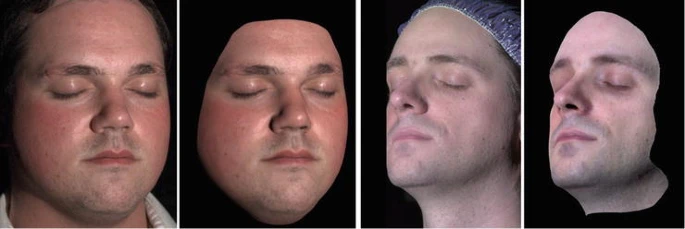
Physically-based models, including Cook-Torrance, He-Torrance, etc., attempt to model physical reality on the theory of microfacets. Representatively, the Cook-Torrance model has been widely used in computer vision and graphics to model the appearance of real world materials. Indeed, it has been successfully applied in computer graphics to model the surface reflectance of human skin as $\mathbf{Fig\ 25}$.
Microfacet Theory: Roughness
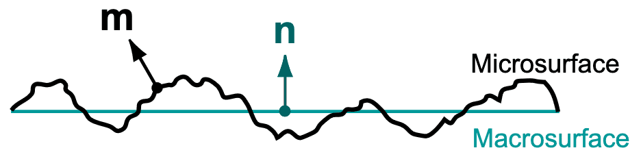
Microfacet theory conceptualize object surfaces as microfacets, a collection of infinitesimal surfaces that are perfectly reflective at a microscopic scale. In microfacet models, a intricate microsurface is substituted with a simplified macrosurface (also referred to as geometric surface) with a modified BSDF that replicates the overall directional scattering of the microsurface. This assumption is grounded in the intuition that the details of the microsurface are too microscopic to be directly observed, thus only the far-field directional scattering pattern is relevant.
Typically geometric optics is assumed and only single scattering is modeled, to circumvent the complexity. Precise modelings of lights such as wave effects and indirect lighting are ignored.
Microfacet Distribution
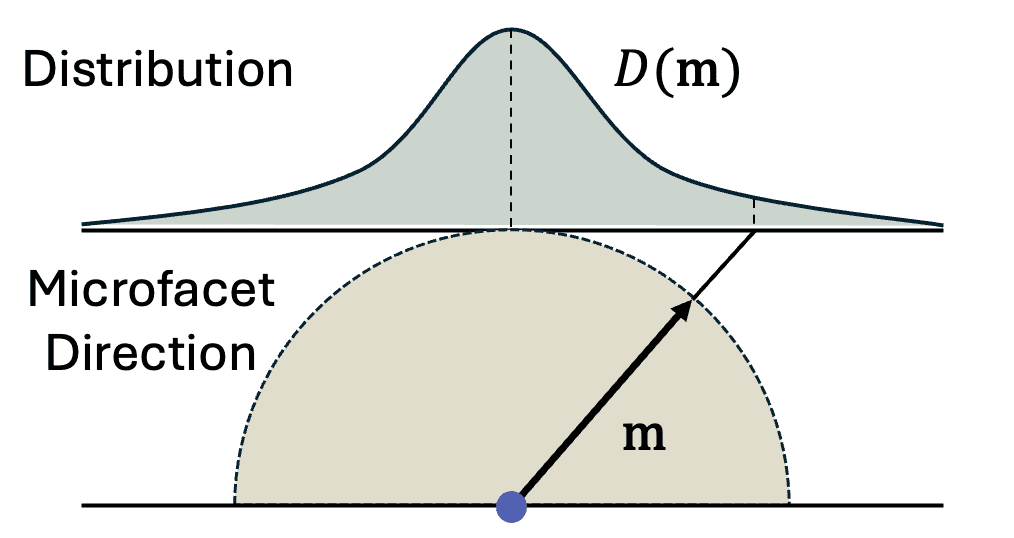
The alignment of microfacets is typically characterized by the distribution function denoted as $D (\mathbf{m})$ that describes the statistical distribution of surface normals $\mathbf{m}$ over the microsurface, which varies depending on the material.
From $\mathbf{Fig\ 26}$, denote the infinitesimal microsurface as $\mathrm{d}A_{\mu}$ with its normal $\mathbf{n}$ and the corresponding simplified macrosurface as $\mathrm{d}A$. It then implies that perpendicular projection of the microsurface exactly covers the macrosurface:
\[\int_{\mathrm{d} A_\mu} (\omega_{m} (\mathrm{p}) \cdot \mathbf{n}) \; \mathrm{d}\mathrm{p} = \int_{\mathrm{d}A} \mathrm{d}\mathrm{p}\]where $\omega_{m} (\mathrm{p})$ is the microfacet normal at point $\mathrm{p}$. However, tracking the orientation of vast numbers of microfacets would be impractical. From this condition that resembles normalization constraint of pdf, we adopt the statistical approach, introducing microfacet distribution function $D(\mathbf{m})$.
Given an infinitesimal solid angle $\mathrm{d} \omega_{\mathrm{m}}$ around $\mathbf{m}$ centered on $\mathbf{m}$, and an infinitesimal macrosurface area $\mathrm{d}A$, $D(\mathbf{m}) \mathrm{d}\omega_{\mathrm{m}} \mathrm{d}A$ defines the portion of the total area of corresponding microsurface $\mathrm{d}A_\mu$ with the surface normal $\mathbf{m}$, denoted as $\mathrm{d}A(\mathbf{m})$: $$ D(\mathbf{m} = \omega_{\mathrm{m}}) := \frac{\mathrm{d}A(\mathbf{m} = \omega_{\mathrm{m}})}{\mathrm{d}\omega_{\mathrm{m}} \mathrm{d}A} \; \left[ \frac{1}{\textrm{sr}} \right] $$ Note that $D (\mathbf{m})$ satisfies the normalization constraint: $$ \int \left(\mathbf{m} \cdot \mathbf{n}\right) \mathrm{d} A\left(\mathbf{m}\right)=\mathrm{d} A \implies \int_{H^2}\left(\mathbf{m} \cdot \mathbf{n}\right) D\left(\mathbf{m}\right) \mathrm{d} \mathbf{m}=1 $$
For example, an ideally smooth macrosurface might possess $D(\mathbf{m}) = \delta (\mathbf{m} - \mathbf{n})$. A physically plausible microfacet distribution should adhere to at least the following simple properties:
- Microfacet density is positive real-valued: $$ 0 \leq D (\mathbf{m}) \leq \infty $$
- Total microsurface area is at least as large as the corresponding macrosurface’s area $\mathrm{d}A$ $$ \mathrm{d}A \leq \int \mathrm{d}A (\mathbf{m}) = \int D(\mathbf{m}) \mathrm{d}\omega_{\mathrm{m}} \mathrm{d}A $$
- The (signed) projected area of the microsurface is the same as the projected area of the macrosurface for any direction $\mathbf{v}$: $$ (\mathbf{v} \cdot \mathbf{n}) \mathrm{d}A = \int (\mathbf{v} \cdot \mathbf{m}) \mathrm{d}A (\mathbf{m}) = \int D(\mathbf{m}) (\mathbf{v} \cdot \mathbf{m}) \mathrm{d}\omega_{\mathrm{m}} \mathrm{d}A $$ It corresponds to the normalization constraint when $\mathbf{v} = \mathbf{n}$.
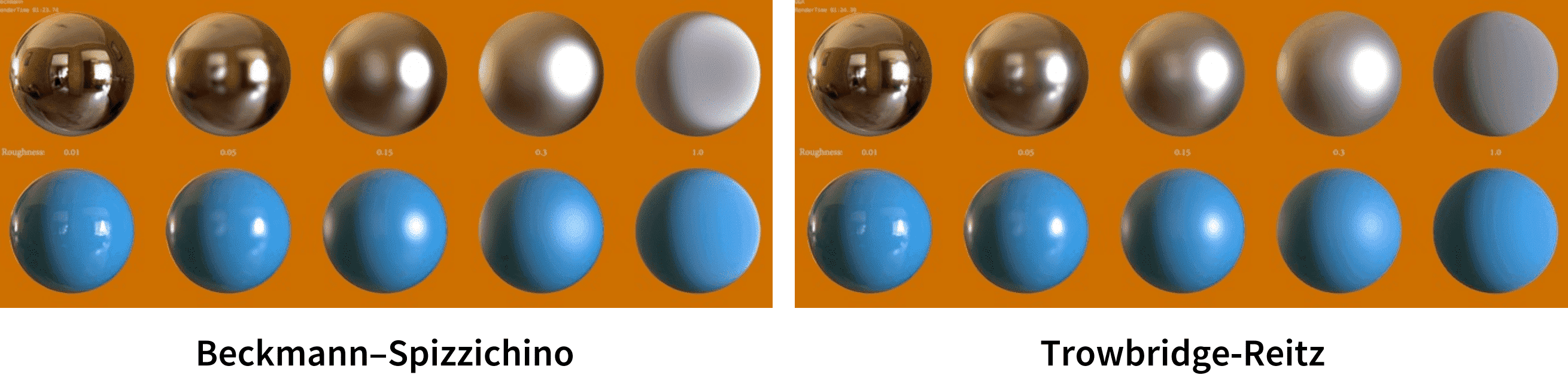
A wide variety of microfacet distribution functions $D$ have been proposed. In this post, we discuss two different represetative distributions called Beckmann-Spizzichino and Trowbridge-Reitz (also called GGX) distribution.
- Beckmann-Spizzichino
The Beckmann-Spizzichino distribution formulates the microfacets as the space of the surface heights $h$ with spherical Gaussian slope: $$ \begin{aligned} - \frac{\mathbf{m}_x}{\mathbf{m}_z} & = \frac{\partial z}{\partial x} \sim \mathcal{N}(0, \alpha^2) \\ - \frac{\mathbf{m}_y}{\mathbf{m}_z} & = \frac{\partial z}{\partial y} \sim \mathcal{N}(0, \alpha^2) \\ \end{aligned} $$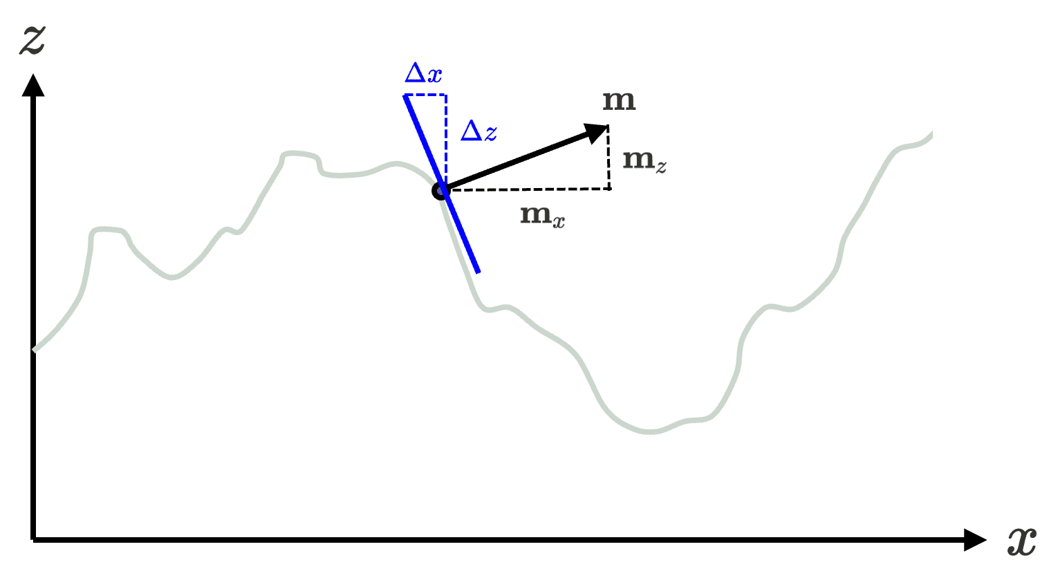
$\mathbf{Fig\ 28.}$ Relationship between surface normal and slope of microfacets
Then, with width parameter $\alpha$, $D(\mathbf{m})$ is modeled as the joint distribution of slopes, i.e. spherical Gaussian: $$ \begin{aligned} D(\mathbf{m}) & \propto \exp \left(-\frac{1}{2}\left[\begin{array}{ll} \frac{\mathbf{m}_x}{\mathbf{m}_z} & \frac{\mathbf{m}_y}{\mathbf{m}_z} \end{array}\right]\left[\begin{array}{cc} \alpha^2 & 0 \\ 0 & \alpha^2 \end{array}\right]^{-1}\left[\begin{array}{l} \frac{\mathbf{m}_x}{\mathbf{m}_z} \\ \frac{\mathbf{m}_y}{\mathbf{m}_z} \end{array}\right]\right) \\ & = \exp \left( -\frac{1}{2\alpha^2} \frac{\mathbf{m}_x^2 + \mathbf{m}_y^2}{\mathbf{m}_z^2}\right) = \exp \left( -\frac{1}{2\alpha^2} \tan^2 \theta_{\mathrm{m}} \right) \end{aligned} $$ where $\mathbf{m} = (\mathbf{m}_x, \mathbf{m}_y, \mathbf{m}_z)$ in coordinate representation and $\mathbf{m} = (\theta_{\mathrm{m}}, \phi_{\mathrm{m}})$ in solid angle representation.
With width parameter $\alpha$ (by omitting the factor for brevity), the complete form of Beckmann-Spizzichino is given by $$ D(\omega_\mathrm{m}) = \frac{e^{\frac{-\tan^2 \theta_{\mathrm{m}}}{\alpha^2}}}{\pi \alpha^2 \cos^4 \theta_{\mathrm{m}}} $$ and is widely used in the optics literature. - Trowbridge-Reitz (GGX)
Another prominent microfacet distribution function is Trowbridge-Reitz (GGX) distribution, which utilizes multivariate $t$-distribution with different scale instead spherical Gaussian distribution: $$ \begin{aligned} D(\mathbf{m}) & \propto \frac{1}{\left(1+\frac{1}{2}\left[\begin{array}{ll} \frac{\mathbf{m}_x}{\mathbf{m}_z} & \frac{\mathbf{m}_y}{\mathbf{m}_z} \end{array}\right]\left[\begin{array}{cc} \alpha_x^2 & 0 \\ 0 & \alpha_y^2 \end{array}\right]^{-1}\left[\begin{array}{c} \frac{\mathbf{m}_x}{\mathbf{m}_z} \\ \frac{\mathbf{m}_y}{\mathbf{m}_z} \end{array}\right]\right)^2} \\ & = \frac{1}{\left(1+\frac{1}{2} \frac{\alpha_y^2 \mathbf{m}_x^2 + \alpha_x^2 \mathbf{m}_y^2}{\alpha_x^2 \alpha_y^2 \mathbf{m}_z^2} \right)^2} \\ & = \frac{1}{\left(1+\frac{1}{2} \frac{\mathbf{m}_x^2 + \mathbf{m}_y^2}{ \mathbf{m}_z^2}\left( \frac{\mathbf{m}_x^2}{\alpha_x^2 (\mathbf{m}_x^2 + \mathbf{m}_y^2)} + \frac{\mathbf{m}_y^2}{\alpha_y^2 (\mathbf{m}_x^2 + \mathbf{m}_y^2)} \right) \right)^2} = \frac{1}{\left(1+\frac{1}{2} \tan^2 \theta_{\mathrm{m}} \left( \frac{\cos ^2 \phi_m}{\alpha_x^2}+\frac{\sin ^2 \phi_m}{\alpha_y^2} \right) \right)^2} \\ \end{aligned} $$ With normalization factor, we then simply obtain: $$ D\left(\omega_m\right)=\frac{1}{\pi \alpha_x \alpha_y \cos ^4 \theta_m\left(1+\tan ^2 \theta_m\left(\frac{\cos ^2 \phi_m}{\alpha_x^2}+\frac{\sin ^2 \phi_m}{\alpha_y^2}\right)\right)^2} $$
Viewed from the perspective of the $t$-distribution being a heavy-tailed Gaussian, the GGX distribution ($t$-distribution) possesses heavier tails than the Beckmann-Spizzichino (Gaussian), thereby leading to increased shadowing effects.

Geometric Attenuation
Several factors determine the scattering result on the surface, and the distribution of microfacet normals alone isn’t enough to fully characterize the microsurface for rendering. Typically, following three scenarios are important geometric effects to take account for modeling microfacet reflection.
- Masking: occlusion by another microfacet
- Shadowing: light does not directly reach the microfacet
- Interreflection: light bounces among the microfacets

Widely employed microfacet BSDFs ignore interreflection effect and instead model the masking and shadowing effects using statistical approximations with efficient evaluation procedures, so we omit the discussion of interreflection in this post.
Masking
Due to backfacing or occulusion by other microfacets, only a subset of microfacets is visible from each view. Denoting the masking function that specifies the fraction of microfacets with surface normal $\mathbf{m}$ that are visible from direction $\omega$ as $G_1 (\omega, \omega_{\mathrm{m}})$, our normalization constraint can be further extended with regard to arbitrary projection as follows:
\[\begin{gathered} \int_{H^2} D\left(\omega_m\right)\left(\omega_m \cdot \mathbf{n}\right) \mathrm{d} \omega_m=1 \\ \Downarrow \\ \int_{H^2} D\left(\omega_m\right) \cdot \color{red}{\underbrace{G_1\left(\omega, \omega_m\right)}_{\text{discard occlusion}}} \cdot \color{blue}{\underbrace{\max \left(0, \omega_m \cdot \omega\right)}_{\text{discard backfacing}}} \; \mathrm{d} \omega_m=\underbrace{\omega \cdot \mathbf{n} = \cos \theta}_{\text{ fraction of visible }} \end{gathered}\]

As the microfacet distribution alone is ambiguous to determine a specific $G(\omega, \omega_{\mathrm{m}})$, an approximation is frequently employed. In this discussion, we explore the commonly used technique known as Smith’s approximation.
Smith simply assumes that the normals of different points on the surface are assumed to be statistically independent, i.e. not autocorrelated. Then the material conceptually turns from a continuous surface to a random discontinuous set of microfacets.
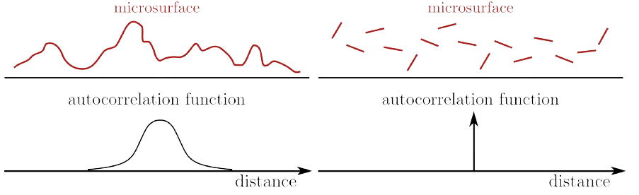
While the surface normal $\omega_{\mathrm{m}}$ pertains to a local attribute of the microfacet, the potential occlusion arises elsewhere on the microsurface, constituting a distant attribute, still on the micro-scale. Given that the microsurface is not autocorrelated, local properties remain independent of distant properties. Consequently, masking becomes independent of the microsurface normal $\omega_{\mathrm{m}}$ with the exception of backfacing facets, which are disregarded ($\omega \cdot \omega_{\mathrm{m}} > 0$): $$ G_1\left(\omega, \omega_m\right) = \chi_{\omega \cdot \omega_{\mathrm{m}} > 0} \cdot G_1 (\omega) $$ Therefore, the masking term can then be moved out of the integral: $$ \begin{gathered} \int_{H^2} D\left(\omega_m\right) G_1\left(\omega, \omega_m\right) \max \left(0, \omega_m \cdot \omega \right) \mathrm{d} \omega_m=\cos \theta \\ \Downarrow \\ \color{green}{G_1(\omega)} \int_{H^2} D\left(\omega_m\right) \max \left(0, \omega_m \cdot \omega \right) \mathrm{d} \omega_m=\cos \theta \end{gathered} $$ And the complete masking function is given by $$ G_1\left(\omega, \omega_m\right) = \chi_{\omega \cdot \omega_{\mathrm{m}} > 0} \cdot \frac{\cos \theta}{\int_{H^2} D\left(\omega_m\right) \max \left(0, \omega_m \cdot \omega \right) \mathrm{d} \omega_m} $$
In wide variety of the literatures, originating from Walter et al. 2007, this Smith masking function is often expressed as a fraction $\frac{1}{1 + \Lambda (\omega)}$ involving a function $\Lambda (\omega)$. This another form of $G_1$ is beneficial in many cases, since it is known as the closed-form solutions for $G_1$ are available for many stochastic surfaces $D(\omega_{\mathrm{m}})$ and pertain to this form. For instance:
-
Beckmann-Spizzichino
$$ G_1 (\omega, \omega_{\mathrm{m}}) = \chi_{\frac{\omega \cdot \mathbf{m}}{\omega \cdot \mathbf{n}} > 0} \cdot \frac{2}{1 + \text{erf}(a) + \frac{1}{a \sqrt{\pi}} e^{-a^2}} $$ where $a = (\alpha \tan \theta)^{-1}$ and $\mathbf{n}$, $\mathbf{m}$ are surface normal of macro- and micro-surface, respectively. -
Trowbridge-Reitz (GGX)
$$ G_1 (\omega, \omega_{\mathrm{m}}) = \chi_{\frac{\omega \cdot \mathbf{m}}{\omega \cdot \mathbf{n}} > 0} \cdot \frac{2}{1 + \sqrt{1 + \alpha^2 \tan^2 \theta}} $$ where $\alpha = \sqrt{\alpha_x^2 \cos^2 \phi + \alpha_y^2 \sin^2 \phi}$.
Masking-Shadowing
The BSDF is a function of two directional arguments: lighting direction $\omega_{\mathrm{i}}$ and view direction $\omega_{\mathrm{o}}$, where each is influenced by occlusion effects, namely masking and shadowing. To account for both scenarios, we extend $G_1 (\omega_{\mathrm{o}}, \omega_{\mathrm{m}})$ into the masking-shadowing function $G_2 (\omega_{\mathrm{o}}, \omega_{\mathrm{i}}, \omega_{\mathrm{m}})$ that provides the fraction of microfacets in a differential area that are simultaneously visible from both directions. Once again, an approximation is necessary.
-
Separable Masking and Shadowing
The simplest and most widely used variant is the separable form popularized by Walter et al. 2007: $$ \begin{aligned} G_2 (\omega_{\mathrm{o}}, \omega_{\mathrm{i}}, \omega_{\mathrm{m}}) & = G_1 (\omega_{\mathrm{o}}, \omega_{\mathrm{m}}) G_1 (\omega_{\mathrm{i}}, \omega_{\mathrm{m}}) \\ & = \frac{\chi_{\omega_{\mathrm{o}} \cdot \omega_{\mathrm{m}} > 0}}{1 + \Lambda (\omega_{\mathrm{o}})} \frac{\chi_{\omega_{\mathrm{i}} \cdot \omega_{\mathrm{m}} > 0}}{1 + \Lambda (\omega_{\mathrm{i}})} \end{aligned} $$ However, this independence assumption is a rather severe approximation that tends to overestimate the extent of shadowing and masking, as some degree of correlation typically exists. Consequently, this can lead to undesirable dark regions in rendered images. -
Height-Correlated Masking and Shadowing
Intuitively, masking and shadowing are correlated through the height of the microfacets: the microfacet is elevated within the microsurface, the greater the likelihood that it will be visible for $\omega_{\mathrm{o}}$ (unmasked) and for $\omega_{\mathrm{i}}$ (unshadowed) simultaneously increases. This height-correlation can be incorporated in the following form: $$ G_2 (\omega_{\mathrm{o}}, \omega_{\mathrm{i}}, \omega_{\mathrm{m}}) = \frac{\chi_{\omega_{\mathrm{o}} \cdot \omega_{\mathrm{m}} > 0} \cdot \chi_{\omega_{\mathrm{i}} \cdot \omega_{\mathrm{m}} > 0}}{1 + \Lambda (\omega_{\mathrm{o}}) + \Lambda (\omega_{\mathrm{i}})} $$ where the precise derivation is given in Heitz et al. 2014.
Please refer to Heitz et al. 2014 for more detail about the approximation of masking-shadowing Function.
Torrance-Sparrow Model
An early microfacet model was developed by Torrance and Sparrow in 1967 to model metallic surfaces. It assumes that the surface is a collection of ideally smooth mirrored microfacets. That is, given the incoming and outgoing ray directions $\omega_{\mathrm{i}}$ and $\omega_{\mathrm{o}}$, only the microfacets that have the half-angle vector as the surface normal will cause ideal specular reflection:
\[\omega_{\mathrm{m}} = \frac{\omega_{\mathrm{i}} + \omega_{\mathrm{o}}}{\lVert \omega_{\mathrm{i}} + \omega_{\mathrm{o}} \rVert}\]The BRDF of Torrance-Sparrow model is given by $$ f_r (\mathrm{p}, \omega_{\mathrm{i}}, \omega_{\mathrm{o}}) = \frac{D(\omega_{\mathrm{m}}) F(\omega_{\mathrm{o}} \cdot \omega_{\mathrm{m}}) G (\omega_{\mathrm{i}}, \omega_{\mathrm{o}})}{4 \cos \theta_{\mathrm{i}} \cos \theta_{\mathrm{o}}} $$ where $\omega_{\mathrm{m}} = \frac{\omega_{\mathrm{i}} + \omega_{\mathrm{o}}}{\lVert \omega_{\mathrm{i}} + \omega_{\mathrm{o}} \rVert}$ is the half-angle vector that equals to the normal vector of reflection to $\omega_{\mathrm{o}}$ from $\omega_{\mathrm{i}}$, $F(\omega_{\mathrm{o}} \cdot \omega_{\mathrm{m}})$ is the Fresnel term based on the angel of incidence, and $G (\omega_{\mathrm{i}}, \omega_{\mathrm{o}})$ is geometric attenuation factor.
$\mathbf{Proof.}$
Consider the differential flux $\mathrm{d} \Phi_{\mathrm{m}}$ incident on the microfacets oriented with half-angle $\omega_{\mathrm{m}}$ for $\omega_{\mathrm{i}}$ and $\omega_{\mathrm{o}}$. From the definition of radiance:
\[\mathrm{d} \Phi_{\mathrm{m}} = L_{\mathrm{i}} (\omega_{\mathrm{i}}) \; \mathrm{d} \omega_{\mathrm{i}} \; \mathrm{d} A(\omega_{\mathrm{m}}) \cos \theta_{\mathrm{m}}\]where $\mathrm{d} A(\omega_{\mathrm{m}})$ is the total area of the microfacets orienting $\omega_\mathrm{m}$ that equals to
\[\mathrm{d} A (\omega_{\mathrm{m}}) = D(\omega_{\mathrm{m}}) \; \mathrm{d} \omega_{\mathrm{m}} \mathrm{d} A\]and $\theta_{\mathrm{m}}$ is the angle between $\omega_{\mathrm{i}}$ and $\omega_{\mathrm{m}}$. Therefore,
\[\mathrm{d} \Phi_{\mathrm{m}} = L_{\mathrm{i}} (\omega_{\mathrm{i}}) \; \mathrm{d} \omega_{\mathrm{i}} \; D(\omega_{\mathrm{m}}) \; \mathrm{d} \omega_{\mathrm{m}} \mathrm{d} A \cos \theta_{\mathrm{m}}\]Assuming that the microfacets individually reflect light according to Fresnel’s law and incorporating the geometric attenuation term $G (\omega_{\mathrm{i}}, \omega_{\mathrm{o}})$, the outgoing flux $\mathrm{d} \Phi_{\mathrm{o}}$ is
\[\mathrm{d} \Phi_{\mathrm{o}} = F(\omega_{\mathrm{o}} \cdot \omega_{\mathrm{m}}) G (\omega_{\mathrm{i}}, \omega_{\mathrm{o}}) \mathrm{d} \Phi_{\mathrm{m}}\]From the definition of the reflected outgoing radiance $L (\omega_{\mathrm{o}})$:
\[L (\omega_{\mathrm{o}}) = \frac{\mathrm{d} \Phi_{\mathrm{o}}}{\mathrm{d}\omega_{\mathrm{o}} \cos \theta_{\mathrm{o}} \; \mathrm{d}A}\]we obtain
\[L (\omega_{\mathrm{o}}) = \frac{F(\omega_{\mathrm{o}} \cdot \omega_{\mathrm{m}}) \; G (\omega_{\mathrm{i}}, \omega_{\mathrm{o}}) \; L_{\mathrm{i}} (\omega_{\mathrm{i}}) \; \mathrm{d} \omega_{\mathrm{i}} \; D(\omega_{\mathrm{m}}) \; \mathrm{d} \omega_\mathrm{m} \; \mathrm{d}A \cos \theta_{\mathrm{m}}}{\mathrm{d}\omega_{\mathrm{o}} \cos \theta_{\mathrm{o}} \; \mathrm{d}A}\]Note that, because $\omega_{\mathrm{i}}$ is computed by reflecting $\omega_{\mathrm{o}}$ about $\omega_{\mathrm{m}}$ and thus $\theta_{\mathrm{i}} = 2\theta_{\mathrm{m}}$, we obtain the following relation:
\[\begin{aligned} \frac{\mathrm{d} \omega_{\mathrm{m}}}{\mathrm{d} \omega_{\mathrm{i}}} & =\frac{\sin \theta_{\mathrm{m}} \mathrm{d} \theta_{\mathrm{m}} \mathrm{d} \phi_{\mathrm{m}}}{\sin 2 \theta_{\mathrm{m}} 2 \mathrm{~d} \theta_{\mathrm{m}} \mathrm{d} \phi_{\mathrm{m}}} \\ & =\frac{\sin \theta_{\mathrm{m}}}{4 \cos \theta_{\mathrm{m}} \sin \theta_{\mathrm{m}}} \\ & =\frac{1}{4 \cos \theta_{\mathrm{m}}} \\ & =\frac{1}{4\left(\omega_{\mathrm{i}} \cdot \omega_{\mathrm{m}}\right)}=\frac{1}{4\left(\omega_{\mathrm{o}} \cdot \omega_{\mathrm{m}}\right)} = \frac{1}{4 \cos \theta_{\mathrm{m}}} = \frac{\mathrm{d} \omega_{\mathrm{m}}}{\mathrm{d} \omega_{\mathrm{o}}}. \end{aligned}\]
Finally, the result is derived:
\[\begin{gathered} f_r (\mathrm{p}, \omega_{\mathrm{i}}, \omega_{\mathrm{o}}) = \frac{L (\omega_{\mathrm{o}})}{L_{\mathrm{i}} (\omega_{\mathrm{i}}) \cos \theta_{\mathrm{i}} \; \mathrm{d} \omega_{\mathrm{i}}} \\ \Downarrow \\ f_r (\mathrm{p}, \omega_{\mathrm{i}}, \omega_{\mathrm{o}}) = \frac{D(\omega_{\mathrm{m}}) F(\omega_{\mathrm{o}} \cdot \omega_{\mathrm{m}}) G (\omega_{\mathrm{i}}, \omega_{\mathrm{o}})}{4 \cos \theta_{\mathrm{i}} \cos \theta_{\mathrm{o}}} \end{gathered}\] \[\tag*{$\blacksquare$}\]Cook-Torrance Model
Cook-Torrance model is an extension of the Torrance-Sparrow model, developed in 1982, that combines a Lambertian diffuse term with a specular term based on microfacet reflections. With constant ratios $s$ and $d$ (i.e. $s + d = 1$) that balances out the diffuse and specular contributions, the BRDF of Cook-Torrance is given by:
$$ \begin{gathered} f_r (\mathrm{p}, \omega_{\mathrm{i}}, \omega_{\mathrm{o}}) = s R_{\mathrm{s}} (\omega_{\mathrm{i}}, \omega_{\mathrm{o}}) + d R_{\mathrm{d}} (\omega_{\mathrm{i}}, \omega_{\mathrm{o}}) \\ \begin{aligned} \text{ where } R_{\mathrm{s}} (\omega_{\mathrm{i}}, \omega_{\mathrm{o}}) & = \frac{D(\omega_{\mathrm{m}}) F(\omega_{\mathrm{o}} \cdot \omega_{\mathrm{m}}) G (\omega_{\mathrm{i}}, \omega_{\mathrm{o}})}{4 \cos \theta_{\mathrm{i}} \cos \theta_{\mathrm{o}}} \\ R_{\mathrm{d}} (\omega_{\mathrm{i}}, \omega_{\mathrm{o}}) & = \frac{\rho_{\mathrm{d}}}{\pi} \end{aligned} \end{gathered} $$
Specifically, the original authors Cook and Torrance employed the following functions for $D$ and $G$, although alternative functions may also be suitable.
\[\begin{gathered} D(\omega_{\mathrm{m}}) = \frac{e^{\frac{-\tan^2 \theta_{\mathrm{m}}}{\alpha^2}}}{\pi \alpha^2 \cos^4 \theta_{\mathrm{m}}} \; (\textrm{Beckmann-Spizzichino}) \\ G (\omega_{\mathrm{i}}, \omega_{\mathrm{o}}) = \min \left\{ 1, \frac{2 (\omega_{\mathrm{m}} \cdot \mathbf{n}) (\omega_{\mathrm{o}} \cdot \mathbf{n})}{\omega_{\mathrm{m}} \cdot \omega_{\mathrm{o}}}, \frac{2 (\omega_{\mathrm{m}} \cdot \mathbf{n}) (\omega_{\mathrm{i}} \cdot \mathbf{n})}{\omega_{\mathrm{m}} \cdot \omega_{\mathrm{o}}} \right\} \end{gathered}\]where $\mathbf{n}$ is the surface normal at point $\mathrm{p}$ and $\omega_{\mathrm{m}}$ is the half-angle vector between $\omega_{\mathrm{i}}$ and $\omega_{\mathrm{o}}$. It’s worth noting that this $G$ is derived from the assumption of V-cavity microsurface that model the roughness with V-shaped groove and is the most common alternative to the Smith’s approximation.
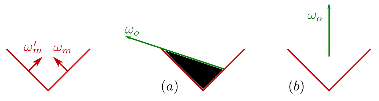
In V-cavity microsurface, for each microfacet (V-shaped groove) have only the two symmetric normals $\omega_{\mathrm{m}}$ and $\omega_{\mathrm{m}}^\prime$. Then, the distribution of normals is given by
\[D(\omega) = \frac{1}{2} \frac{\delta (\omega - \omega_{\mathrm{m}})}{\omega_{\mathrm{m}} \cdot \mathbf{n}} + \frac{1}{2} \frac{\delta (\omega - \omega_{\mathrm{m}}^\prime)}{\omega_{\mathrm{m}}^\prime \cdot \mathbf{n}}\]with the normalization constraint
\[\int_{H^2} (\omega \cdot \mathbf{n}) D (\omega) \; \mathrm{d}\omega = \frac{1}{2} + \frac{1}{2} = 1.\]Then, by definition of masking function $G_1$:
\[\begin{aligned} \cos \theta_{\mathrm{o}} = \omega_{\mathrm{o}} \cdot \mathbf{n} & = \int_{H^2} G_1 (\omega_{\mathrm{o}}, \omega) \; (\omega \cdot \omega_\mathrm{o}) D(\omega) \; \mathrm{d} \omega \\ & = \frac{1}{2} G_1 (\omega_{\mathrm{o}}, \omega_{\mathrm{m}}) \frac{\omega_{\mathrm{o}} \cdot \omega_{\mathrm{m}}}{\omega_{\mathrm{m}} \cdot \mathbf{n}} + \frac{1}{2} G_1 (\omega_{\mathrm{o}}, \omega_{\mathrm{m}}^\prime) \frac{\omega_{\mathrm{o}} \cdot \omega_{\mathrm{m}}^\prime}{\omega_{\mathrm{m}}^\prime \cdot \mathbf{n}} \end{aligned}\]From the appearance of the V-shape, there are only two possible scenarios consdering masking; two surfaces are visible simulatenously, i.e. both $G_1 (\omega_{\mathrm{o}}, \omega_{\mathrm{m}})= 1$ and $G_1 (\omega_{\mathrm{o}}, \omega_{\mathrm{m}}^\prime)= 1$, or only one surface is visible. In latter case, we have
\[\cos \theta_{\mathrm{o}} = \frac{1}{2} G_1 (\omega_{\mathrm{o}}, \omega_{\mathrm{m}}) \frac{\omega_{\mathrm{o}} \cdot \omega_{\mathrm{m}}}{\omega_{\mathrm{m}} \cdot \mathbf{n}}\]which leads to
\[G_1 (\omega_{\mathrm{o}}, \omega_{\mathrm{m}}) = \frac{2 \cos \theta_{\mathrm{o}} \; (\omega_{\mathrm{m}} \cdot \mathbf{n})}{\omega_{\mathrm{o}} \cdot \omega_{\mathrm{m}}} = \frac{2 (\omega_{\mathrm{o}} \cdot \mathbf{n}) (\omega_{\mathrm{m}} \cdot \mathbf{n})}{\omega_{\mathrm{o}} \cdot \omega_{\mathrm{m}}}\]
Analogously, we can obtain the shadowing function by substituting $\omega_{\mathrm{o}}$ by $\omega_{\mathrm{i}}$:
\[G_1 (\omega_{\mathrm{i}}, \omega_{\mathrm{m}}) = \frac{2 \cos \theta_{\mathrm{i}} \; (\omega_{\mathrm{m}} \cdot \mathbf{n})}{\omega_{\mathrm{o}} \cdot \omega_{\mathrm{m}}} = \frac{2 (\omega_{\mathrm{i}} \cdot \mathbf{n}) (\omega_{\mathrm{m}} \cdot \mathbf{n})}{\omega_{\mathrm{o}} \cdot \omega_{\mathrm{m}}}\]Note that $\omega_{\mathrm{m}} \cdot \omega_{\mathrm{i}} = \omega_{\mathrm{m}} \cdot \omega_{\mathrm{o}}$. The result of these two configurations can be expressed in a single formula:
\[G (\omega_{\mathrm{i}}, \omega_{\mathrm{o}}) = \min \left\{ 1, \frac{2 (\omega_{\mathrm{m}} \cdot \mathbf{n}) (\omega_{\mathrm{o}} \cdot \mathbf{n})}{\omega_{\mathrm{m}} \cdot \omega_{\mathrm{o}}}, \frac{2 (\omega_{\mathrm{m}} \cdot \mathbf{n}) (\omega_{\mathrm{i}} \cdot \mathbf{n})}{\omega_{\mathrm{m}} \cdot \omega_{\mathrm{o}}} \right\}\]Reference
[1] Huges et al. “Computer Graphics: Principles and Practice (3rd ed.)” (2013).
[2] Shirley et al. “Fundamentals of computer graphics” AK Peters/CRC Press, 2009.
[3] Matt Pharr, Wenzel Jakob, and Greg Humphreys, “Physically Based Rendering: From Theory To Implementation”
[4] How Do We See Light? | Ask A Biologist
[5] SIGGRAPH 2014 Course: Physically Based Shading in Theory and Practice
[6] Giancoli, Douglas C. “Physics: Principles with Applications -Standalone book.” (2013).
[7] Edmund optics, “Introduction to Polarization”
[8] Matthew Schwartz, “Lecture 15: Refraction and Reflection”, Harvard
[9] Cornell University, “Fresnel Reflectance”
[10] Schlick, C. An inexpensive BRDF model for physically-based rendering. Computer Graphics Forum, 13(3):233–246, 1994. DOI: 10.1111/1467-8659.1330233
[11] LearnOpenGL, “Advanced Lighting”
[12] F. Giesen, “Phong Normalization Factor derivation,” 2009
[13] E. P. Lafortune and Y. D. Willems, “Using the modified phong reflectance model for physically based rendering,” 1994
[14] Computer Graphics Stack Exchange, “Phong and the Rendering Equation: What’s with the cosine?”
[15] C. Schüler, “An efficient and Physically Plausible Real Time Shading Model,” in ShaderX7, 2009.
[16] Dutre, Philip, Philippe Bekaert, and Kavita Bala. Advanced global illumination. AK Peters/CRC Press, 2018.
[17] Walter et al. “Microfacet Models for Refraction through Rough Surfaces”, Eurographics Symposium on Rendering (2007)
[18] Heitz et al. “Understanding the masking-shadowing function in microfacet-based BRDFs.” Journal of Computer Graphics Techniques 3.2 (2014): 32-91.
[19] Nathan Reed, “Slope Space in BRDF Theory”
[20] Wikipedia, “Subsurface scattering”
Leave a comment