
[Graphics] Volume Rendering
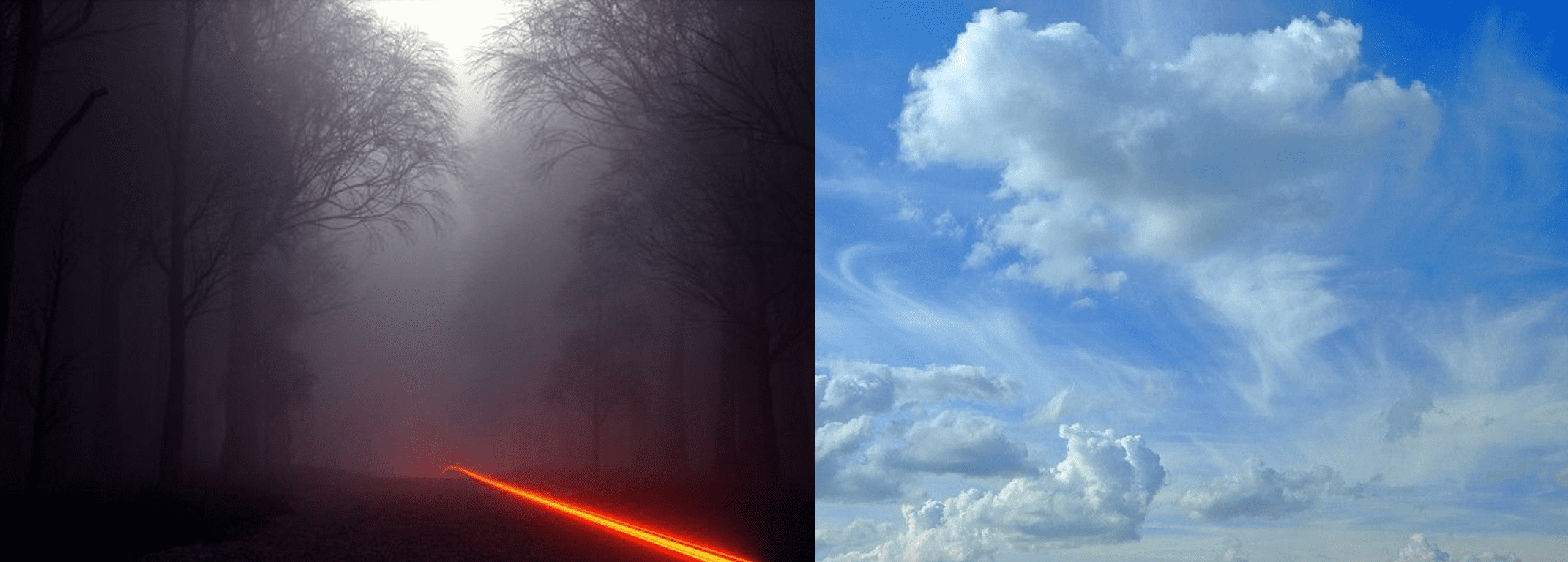
We have assumed so far that scenes consist of collections of surfaces in a vacuum, implying that radiance remains constant along rays between surfaces. However, this assumption turns out to be inaccurate in a wide variety of real-world scenarios, where numerous visual effects exhibit volumetric characteristics. For example, fog and smoke attenuate and scatter light, and scattering from particles in the atmosphere makes the sky blue and sunsets red (known as Rayleigh scattering). These effects pose challenges for modeling with the simple surface renderings we’ve discussed thus far.
Volume rendering (here, the term volume technically denotes participating media-large numbers of minuscule particles distributed throughout 3D region) aims to model such volumetric phenomena and also visualize 2D projection of 3D sampled datasets, including data acquired via medical imaging devices (e.g. CT, MRI) or computational fluid dynamics simulations. This post introduces the mathematics that describe how traveling rays are emitted, absorbed, and scattered by participating media.
Volume Scattering Models
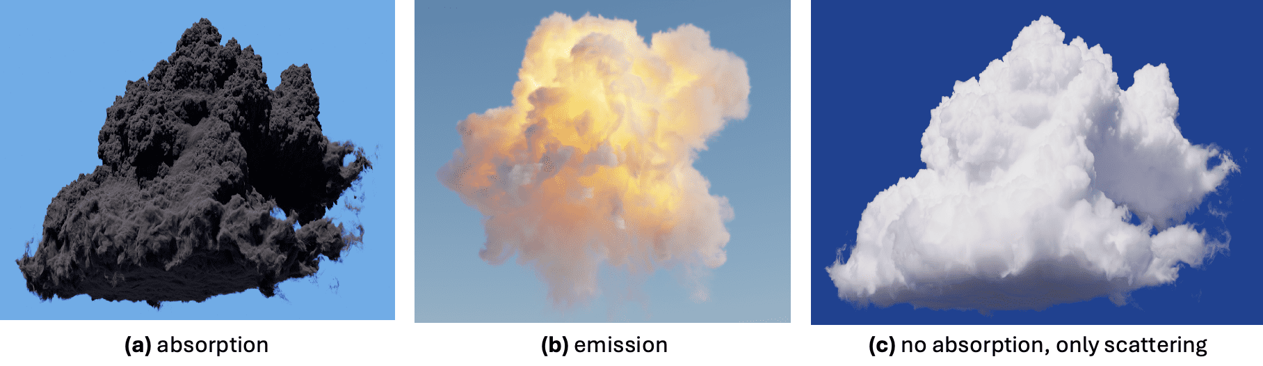
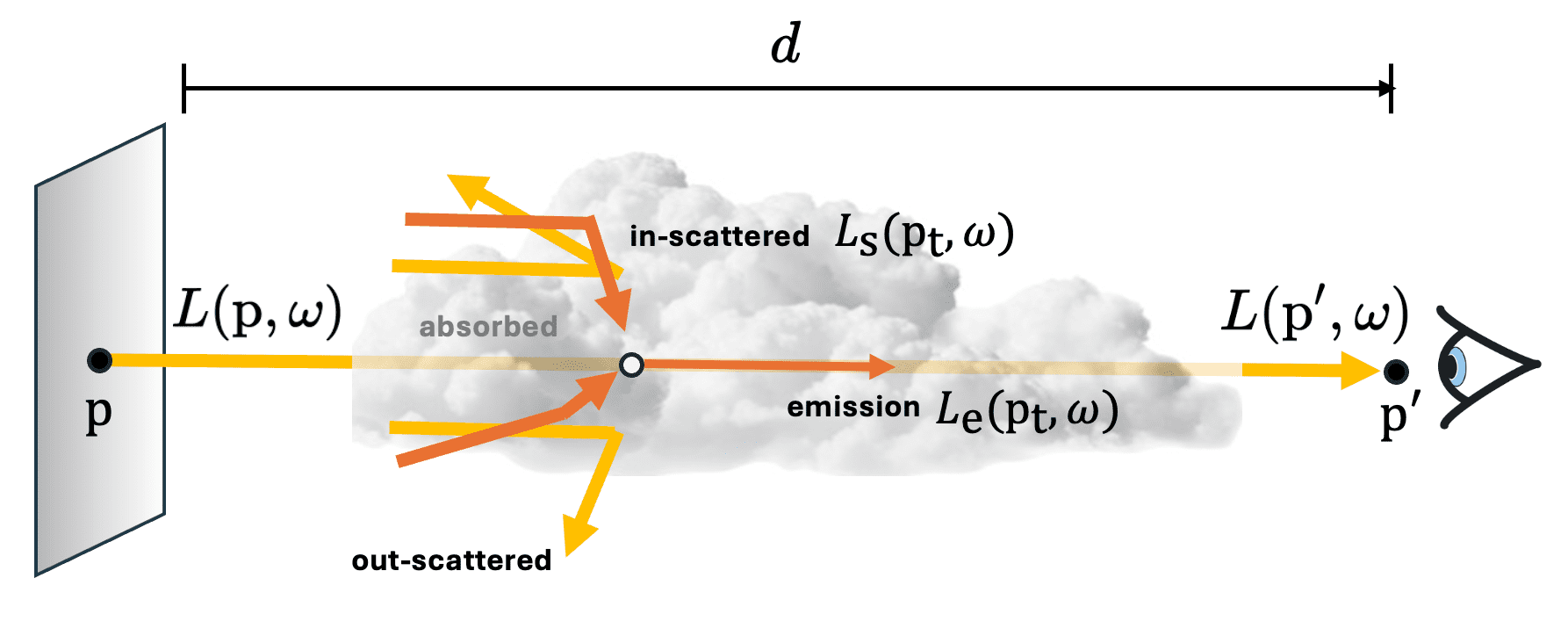
Typically, there are three main physical phenomena that affect the distribution of radiance in an environment with participating media:
- Absorption: the reduction in radiance due to the conversion of light to another form of energy, such as heat.
- Emission: radiance that is added to the environment from luminous particles.
- Scattering: radiance heading in one direction that is scattered to other directions due to collisions with particles.
Absorption
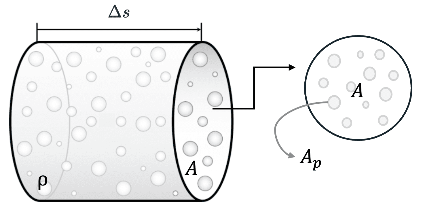
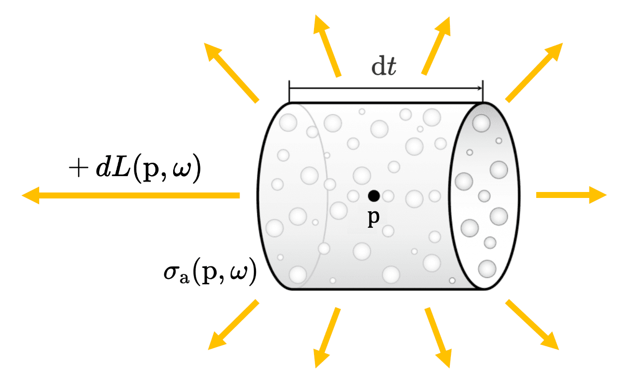
Consider a cylindrical volume of medium filled with randomly distributed absorbing particles at a density of $\rho$ particles per unit volume. As shown in Figure 3, let $A_p$ be the average projected area of the particles onto the face of cylinder. As viewed from the direction of propagation, particles thus block a fraction of the area:
\[\frac{\rho A \Delta s A_p}{A}\]
Therefore the radiance transmitted through the interval $\Delta s$ is given by
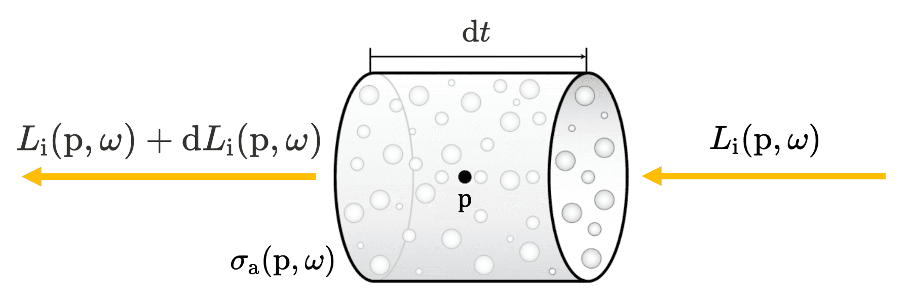
\[\begin{gathered} L (\mathrm{p} + \omega \Delta s, \omega) = (1 - \rho \Delta s A_p) L (\mathrm{p}) \\ \therefore \frac{\mathrm{d} L(\mathrm{p}, \omega)}{\mathrm{d}s} = - \rho A_p L(\mathrm{p}, \omega) \end{gathered}\]Here, the term $\rho A_p$ with reciprocal distance unit $\mathrm{m}^{-1}$ is known as the medium’s absorption coefficient and denotes as $\sigma_{\mathrm{a}}$. It describes the probability density that light is absorbed per unit distance traveled in the medium. With the center $\mathrm{p}$ of infinitesimal cylinder and the direction $\omega$ of incident radiance, we model the absorption effect as follows:
\[\mathrm{d} L_{\mathrm{i}} (\mathrm{p}, \omega) := -\sigma_{\mathrm{a}} (\mathrm{p}, \omega) L_{\mathrm{i}} (\mathrm{p}, \omega) \; \mathrm{d}t\]
By solving the differential equation, it is possible to obtain the total amount of survived incident radiance when the ray travels a distance $d$ in direction $\omega$ through the medium starting at $\mathrm{p}$:
\[L_{\mathrm{i}} (\mathrm{p} + \omega d, \omega) = \exp \left( \int_0^{d} - \sigma_{\mathrm{a}} (\mathrm{p} + t \omega, \omega) \; \mathrm{d}t \right) \cdot L_{\mathrm{i}} (\mathrm{p}, \omega)\]Emission
In contrast, emission increases the radiance of incoming ray due to chemical, thermal, or nuclear processes that convert energy into visible light, while absorption reduces the amount of radiance. In general, grounded on the Kirchhoff’s law of thermal radiation, the emission is also modeled using absorption coefficient; the change in radiance due to emission is given by
\[\mathrm{d}L (\mathrm{p}, \omega) = \sigma_{\mathrm{a}} (\mathrm{p}, \omega) L_{\mathrm{e}} (\mathrm{p}, \omega)\]Note that it incorporates the assumption of geometric optics that the combined effect of light from various sources always equals the sum of the effects of each light individually. Thus the added radiance $\mathrm{d}L$ is computed with the emitted light $L_{\mathrm{e}}$ only and not dependent on the incoming light $L_{\mathrm{i}}$.
Scattering
As a ray passes through a medium, it may collide with particles and be absorbed, or scattered in different directions. This has two effects on the total radiance that the beam carries. It reduces the radiance exiting a differential region of the beam because some of it is deflected to different directions. Or, it increases the radiance since radiance from other rays may be scattered into the path of the current ray. These effects are called out-scattering and in-scattering, respectively.
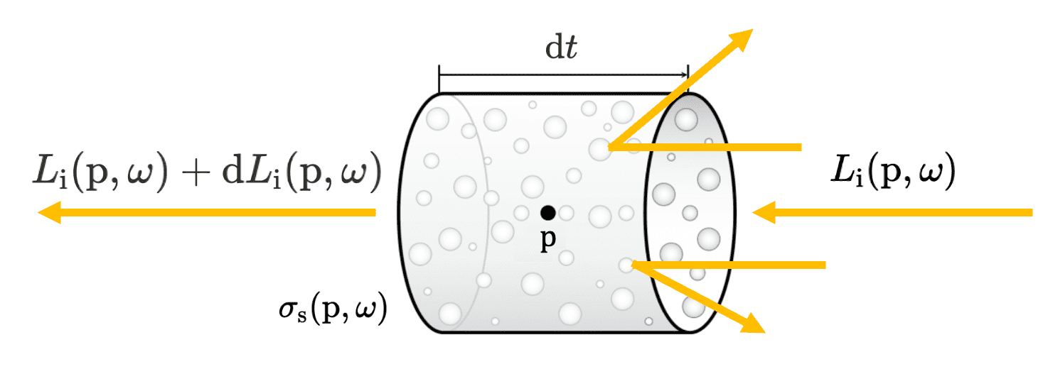
Out-scattering
Given that both absorption and scattering arise from collisions of photons, scattering can similarly be modeled, albeit with a distinct coefficient $\sigma_{\mathrm{s}}$ called scattering coefficient that indicates the probability of out-scattering event occurring per unit distance:
\[\mathrm{d} L_{\mathrm{i}} (\mathrm{p}, \omega) := -\sigma_{\mathrm{s}} (\mathrm{p}, \omega) L_{\mathrm{i}} (\mathrm{p}, \omega) \; \mathrm{d}t\]The only difference lies in the fact that the scattered light contributes to the radiance of other directions, whereas absorbed light just dissipates entirely. The contributions to other rays are quantified through in-scattering.
The total reduction in radiance due to absorption and out scattering is called attenuation or extinction, with the attenuation coefficient $\sigma_{\mathrm{t}}$:
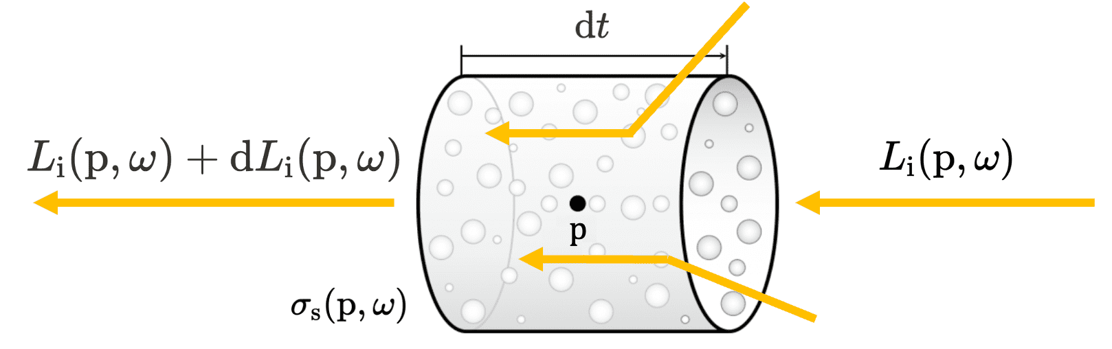
\[\sigma_{\mathrm{t}} (\mathrm{p}, \omega) := \sigma_{\mathrm{a}} (\mathrm{p}, \omega) + \sigma_{\mathrm{s}} (\mathrm{p}, \omega)\]In-scattering
In contrast, scattering from other directions can increase the radiance along an incoming direction. This effect is called in-scattering. The major challenge of quantifying this effect is that the photons are scattered in random directions. In the theory of atmospheric radiation, the phase function $f_{p} (\mathbf{x}, \omega, \omega^\prime)$ describes the angular distribution at point of scattered radiation $\mathbf{x}$, from the incoming radiance along $\omega$ at a point $\mathbf{x}$.
The phase function is the fraction of the intensity (radiance) along the direction $\omega^\prime$ relative to the normalized integral of the scattered intensity at all angles. file:///Users/leeyngdo/Downloads/phase_function_report.pdf
Thus, $f_p$ can be thought of as a probability density function. This leads to the normalization condition:
\[\forall \omega \in \Omega: \; \int_{S^2} f_p (\mathbf{x}, \omega, \omega^\prime) \; d\omega^\prime = 1\]Then, it is possible to model the in-scattering effect with the scattering coefficient $\sigma_{\mathrm{s}}$ that indicates the probability density of scattering event:
\[\mathrm{d}L_\mathrm{i} (\mathrm{p}, \omega) = \sigma_{\mathrm{s}} (\mathrm{p}, \omega) \int_{S^2} f_p (\mathrm{p}, \omega, \omega^\prime) L_{\mathrm{i}} (\mathrm{p}, \omega^\prime) \; \mathrm{d} \omega^\prime\]This term is sometimes referred to as the source term in literatures.
A wide variety of models for phase function have been developed in the literature. Typically, participating medium can exhibit two types of scattering behavior:
- Isotropic (Symmetric): all directions within the sphere are equally likely to be chosen.
- Anisotropic (Asymmetric): certain directions within the sphere of directions are more likely to be chosen than others.
In case of an isotropic medium, the phase function is given by
\[f_{p} (\mathbf{x}, \omega, \omega^\prime) = \frac{1}{4\pi}\]For anisotropic medium, one of the widely used phase functions is the Henyey-Greenstein phase function, which was empirically derived to model the scattering of light by intergalactic dust. It is defined as follows, only depending on the angle $\theta$:
\[f_{p, \textrm{HG}} (\mathbf{x}, \omega, \omega^\prime) = \frac{1}{4\pi} \frac{1 - g^2}{(1 + g^2 + 2g(\cos \theta))^{3/2}}\]where a single parameter $g \in [-1, 1]$ is the asymmety parameter that controls the relative strength of forward and backward scattering as shown in the Figure 8.
Transmittance (Beer–Lambert Law)
When we render a 3D scene, we are usually interested in their aggregate effects on radiance along a ray, which leads to the integral equations rather than local effects at point $\mathrm{p}$ and direction $\omega$ with integro-differential equation. To do so, we first elucidate the reduction in radiance between two points on a ray due to extinction.
Consider the radiance $L (\mathrm{p}, \omega)$ that incidents into the medium with the attenuation coefficient $\sigma_{\mathrm{t}} (\mathrm{p}, \omega)$. Then, the change of radiance when taking a differential step $\mathrm{d}t$ is obtained as follows from our models:
\[L (\mathrm{p} + \omega \cdot \mathrm{d}t, \omega) - L (\mathrm{p}, \omega) = \mathrm{d} L (\mathrm{p}, \omega) = - \sigma_{\mathrm{t}} (\mathrm{p}, \omega) \cdot L (\mathrm{p}, \omega) \cdot \mathrm{d}t\]That is,
\[\begin{gathered} \frac{\mathrm{d} L (\mathrm{p}, \omega) / \mathrm{d} t}{L (\mathrm{p}, \omega)} = - \sigma_{\mathrm{t}} (\mathrm{p}, \omega) \\ \Downarrow \\ \int_0^d \frac{\mathrm{d} L (\mathrm{p} + \omega t, \omega) / \mathrm{d} t}{L (\mathrm{p} + \omega t, \omega)} \; \mathrm{d} t = - \int_0^d \sigma_{\mathrm{t}} (\mathrm{p} + \omega t, \omega) \; \mathrm{d} t \end{gathered}\]This leads to the following equation that indicates the amount of remaining radiance when reaching the new point $\mathrm{p}^\prime = \mathrm{p} + \omega d$ passing through the medium:
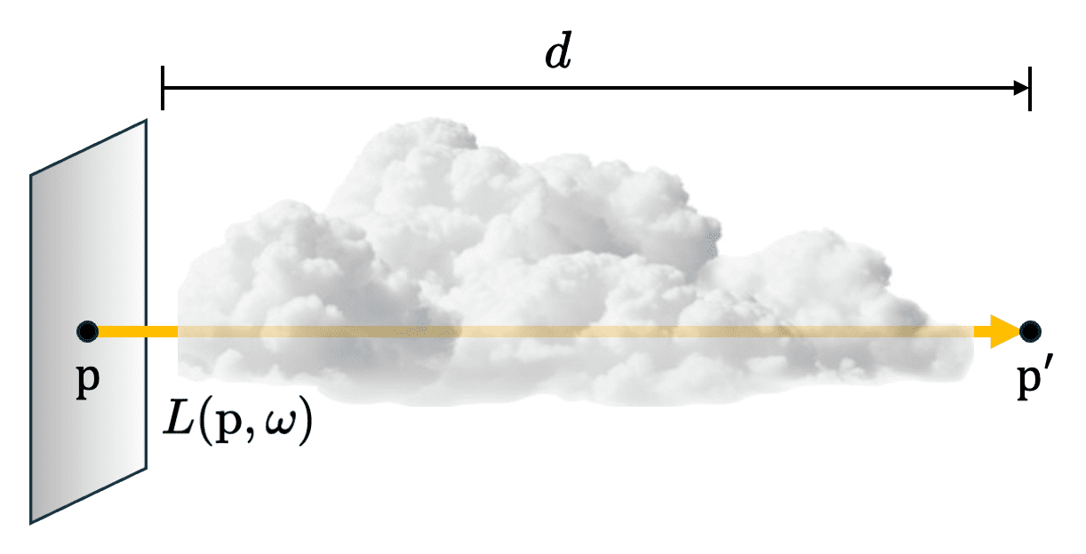
\[\begin{gathered} \log L (\mathrm{p} + \omega t, \omega) \vert_{t = 0}^{t = d} = - \int_0^d \sigma_{\mathrm{t}} (\mathrm{p} + \omega t, \omega) \; \mathrm{d}t \\ \Downarrow \\ L (\mathrm{p}^\prime, \omega) = \exp \left( - \int_0^d \sigma_{\mathrm{t}} (\mathrm{p} + \omega t, \omega) \; \mathrm{d}t \right) \cdot L (\mathrm{p}, \omega) \end{gathered}\]We define the multiplicative term of the last equation as transmittance $\mathcal{T} (\mathrm{p} \to \mathrm{p}^\prime)$, which denotes the fraction of radiance transimitted from $\mathrm{p}$ to $\mathrm{p}^\prime$:
The transmittance between two points $\mathrm{p}$ and $\mathrm{p}^\prime = \mathrm{p}$, denoted as $\mathcal{T} (\mathrm{p} \to \mathrm{p}^\prime)$, is defined by $$ \mathcal{T} (\mathrm{p} \to \mathrm{p}^\prime) \equiv \exp \left( - \int_0^d \sigma_{\mathrm{t}} (\mathrm{p} + \omega t, \omega) \; \mathrm{d}t \right) $$ where $d = \lVert \mathrm{p}^\prime - \mathrm{p} \rVert$ and $\omega = ( \mathrm{p}^\prime - \mathrm{p} ) / d$. And in optics, the negated exponent in the definition is called the optical thickness, or optical depth between the two points $\mathrm{p}$ and $\mathrm{p}^\prime$: $$ \tau (\mathrm{p} \to \mathrm{p}^\prime) \equiv \int_0^d \sigma_{\mathrm{t}} (\mathrm{p} + \omega t, \omega) \; \mathrm{d}t $$ The term originates from the relation that as the optical depth increases, the extent of absorption also amplifies.
Note that the transmittance is defined as a non-increasing function. It aligns with the physical concept that transparency cannot be increased over time along a ray. And here are a few remarks with regard to transimittance:
-
Multiplicative
From the linearity of integral, we obtain $$ \mathcal{T} (\mathrm{p} \to \mathrm{p}^{\prime \prime}) = \mathcal{T} (\mathrm{p} \to \mathrm{p}^{\prime}) \mathcal{T} (\mathrm{p}^\prime \to \mathrm{p}^{\prime \prime}) $$ -
Beer-Lambert Law
When we assume the homogeneous volume, i.e. $\sigma_{\mathrm{t}} (\mathrm{p}, \omega) = \sigma_{\mathrm{t}}$ constant, the formula reduces to $$ \mathcal{T} (\mathbf{x} \to \mathbf{y}) = \exp \left( -\sigma_{\mathrm{t}} \lVert \mathbf{y} - \mathbf{x} \rVert \right). $$ This aligns with the Beer-Lambert law that earticulates the remaining radiance after travesing a finite distance through a medium with a constant extinction coefficient $\sigma_{\mathrm{t}}$.
Radiative Transform Equation (RTE) & Volume Rendering Equation
Given the four volume scattering models, described in the previous sections we can construct a comprehensive model articulating the behavior light in a participating medium. The total change in radiance along the ray at a position $\mathrm{p}$ with direction $\omega$ can be expressed as:
\[\frac{\mathrm{d} L(\mathrm{p}, \omega)}{\mathrm{d}t}= \underbrace{-\underbrace{\sigma_a(\mathbf{x}) L (\mathrm{p}, \omega)}_{\text {absorption }}-\underbrace{\sigma_s(\mathbf{x}) L (\mathrm{p}, \omega)}_{\text {out-scattering }}}_{\text{extinction}} +\underbrace{\sigma_a(\mathbf{x}) L_{\mathrm{e}}(\mathrm{p}, \omega)}_{\text {emission }}+\underbrace{\sigma_{\mathrm{s}} (\mathrm{p}, \omega) \int_{S^2} f_p (\mathrm{p}, \omega, \omega^\prime) L (\mathrm{p}, \omega^\prime) \; \mathrm{d} \omega^\prime}_{\text {in-scattering }} .\]This equation is known as the differential form of the radiative transfer, also called radiative transport equation (RTE), proposed by Chandrasekhar, 1960. For brevity, denote
\[L_{\mathrm{s}} (\mathrm{p}, \omega) = \int_{S^2} f_p (\mathrm{p}, \omega, \omega^\prime) L (\mathrm{p}, \omega^\prime) \; \mathrm{d} \omega^\prime.\]Consider the following non-homogeneous ODE
\[\begin{aligned} & y^\prime + p(x) y = q(x) \\ \text{ where } & p(x)y \equiv \sigma_{\mathrm{t}} (\mathrm{p}, \omega) L(\mathrm{p}, \omega) \\ & q(x) \equiv \sigma_{\mathrm{a}} (\mathrm{p}, \omega) L_{\mathrm{e}} (\mathrm{p}, \omega) + \sigma_{\mathrm{s}} (\mathrm{p}, \omega) L_{\mathrm{s}} (\mathrm{p}, \omega) \end{aligned}\]which yields the solution
\[y(x) = e^{- \int p(x) \mathrm{d}x} \left[\int e^{ - \int p(x) \mathrm{d}x} q(x) \mathrm{d}x + C \right]\]By replacing the $p$ and $q$ terms with their counterparts from the radiative transfer equation and boundary condition $d = 0$ (i.e. $\mathrm{p}^\prime = \mathrm{p} + \omega d = \mathrm{p}$), we obtain
\[L(\mathrm{p}^\prime, \omega) = \int_{0}^{d} \mathcal{T} (\mathrm{p} \to \mathrm{p}_t) \left[ \sigma_{\mathrm{a}} (\mathrm{p}_t, \omega) L_{\mathrm{e}} (\mathrm{p}_t, \omega) + \sigma_{\mathrm{s}} (\mathrm{p}_t, \omega) L_{\mathrm{s}} (\mathrm{p}_t, \omega) \right] \mathrm{d}t + \mathcal{T} (\mathrm{p} \to \mathrm{p}^\prime) L (\mathrm{p}, \omega)\]where \(\mathrm{p}^t = \mathrm{p} + \omega t\). We finally obtain the complete integral equation of the radiance $L( \mathrm{p}, \omega)$ which is known as volume rendering equation:
\[\begin{aligned} L(\mathrm{p}^\prime, \omega) = & \underbrace{\mathcal{T} (\mathrm{p} \to \mathrm{p}^\prime) L (\mathrm{p}, \omega) }_{\text {reduced radiance}} \; + \\ & \underbrace{\int_0^d \mathcal{T} (\mathrm{p} \to \mathrm{p}_t)\sigma_{\mathrm{a}} (\mathrm{p}_t, \omega) L_{\mathrm{e}} (\mathrm{p}_t, \omega) \mathrm{d}t }_{\text {accumulated emitted radiance }} \; + \\ & \underbrace{\int_0^d \mathcal{T} (\mathrm{p} \to \mathrm{p}_t) \sigma_{\mathrm{s}} (\mathrm{p}_t, \omega) \left( \int_{S^2} f_p (\mathrm{p}_t, \omega, \omega^\prime) L (\mathrm{p}_t, \omega^\prime) \mathrm{d}\omega^\prime \right) \mathrm{d}t}_{\text {accumulated in-scattered radiance }} \end{aligned}\]
Reference
[1] Matt Pharr, Wenzel Jakob, and Greg Humphreys, “Physically Based Rendering: From Theory To Implementation”
[2] Nelson Max and Min Chen. Local and global illumination in the volume rendering integral. Technical report, Schloss Dagstuhl, Leibniz Center for Informatics (Germany), 2010.
[3] Tagliasacchi et al. “Volume Rendering Digest (for NeRF)”
[4] Steve Marschner, “Volume light transport”, Cornell University CS 6630 Fall 2015
[5] Ross Bannister, “The Radiative Transfer Equation”
[6] ScratchPixel, “Volume Rendering”
[7] Wojciech Jarosz’s thesis
[8] Liou, K. N., 2002. “An Introduction to Atmospheric Radiation”. Academic Press c/o Elsevier Science, San Diego, CA.
[9] Wikipedia, “Beer-Lambert Law”
Leave a comment