[Graphics] Gaussian Splatting

The advent of NeRF has garnered significant attention in the domain of novel view synthesis, substantially enhancing the quality of synthesis outcomes. Nevertheless, the low training and rendering speed of NeRF impedes its practical application in industries such as VR/AR.

Despite a plethora of efforts in the literatures have been attempted to accelerate the process, it remains challenging to find a robust method capable of both training NeRF quickly enough on a consumer-level GPUs and rendering a 3D scene at an interactive frame rate on common devices such as cellphones and laptops. 3D Gaussian Splatting (3DGS), introduced in Kerbl et al. SIGGRAPH 2023, has emerged as an faster alternative to NeRF with comparable synthesis quality, realizing the low-cost, real-time 3D content creation possible.

Point-Based Graphics

The background of Gaussian Splatting originates from the realm of point-based rendering.

The Rise of Point-Based Graphics

In numerous computer graphics applications, (triangle) meshes are typically the most common surface representation due to their simplicity and flexibility, since surfaces of any shape and topology can be represented by the collection of single mesh. However, meshes may not be suitable in modern computers, as they are becoming increasingly complex while the typical screen resolution does not grow at the same pace.

The explosion of CPUs and graphics hardware performance, and the efficient memory result in the process of vast amounts of highly detailed geometric data. Consequently, 3D models consisting of several millions of meshes are commonplace nowadays. When the number of triangles exceeds the accommodable number of pixels on the screen, rendering such massive datasets leads to be extremely inefficient since triangles of which projected area on the screen is less than one pixel.

$\mathbf{Fig\ 1.}$ Performance of 3D hardware exploded around 2000. GeForce4 is capable of processing 136 million vertices per second (source: Matthias Zwicker)

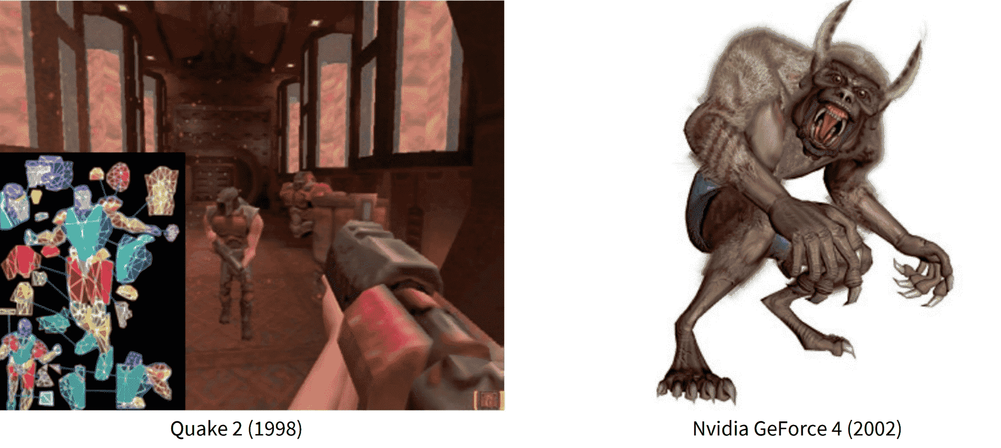
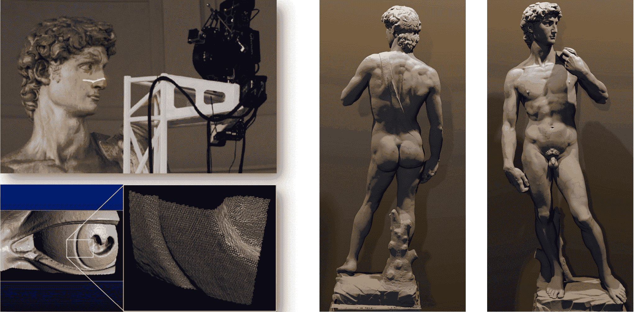
Against this backdrop of accelerating progress, researchers began to explore alternative geometric primitives. And point-based rendering, initially proposed by Levoy and Whitted in 1985, was resurrected primarily due to the work of Levoy et al. SIGGRAPH 2002, titled “The Digital Michelangelo Project: 3D Scanning of Large Statues”.

$\mathbf{Fig\ 2.}$ The high-quality scanned results surprised the field of graphics. (source: Matthias Zwicker)

Surfel: Point Sample Attributes

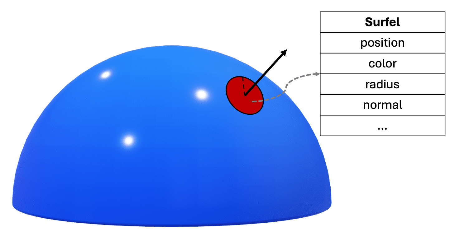
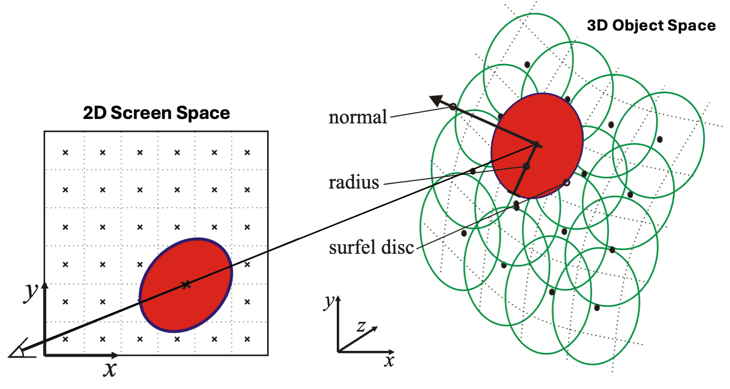
Point-based rendering can be conceptualized as surface reconstruction from its point samples: given a point set, the rendering algorithm aims to transform it into a smooth surface.

Each point sample is characterized by its position, surface normal and shading attributes such as color at the corresponding surface point. If an area is assigned to the point sample, meaning that a surface point is treated as a disk, it is termed a surface element, or surfel in the domain of point-based rendering. Intuitively, the surfel areas must fully cover the surface to ensure a hole-free reconstruction.

$\mathbf{Fig\ 3.}$ Surfel Attributes

Point Rendering Pipeline

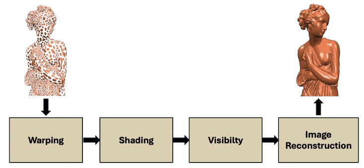
Similar with rasterization, the point rendering pipeline processes point data as follows:

1. Forward Warping
   This stage projects each point to screen space using perspective projection. This is analogous to projecting triangle vertices to image space.
2. Shading
   Per-point shading is performed, any local shading model is applicable. Shading is often performed after visibility (only visible points are shaded) or after image reconstruction using interpolated point attributes (per-pixel shading).
3. Visibility & Reconstruction
   These two stages form a view dependent surface reconstruction in screen space, which is similar to triangle rasterization.

$\mathbf{Fig\ 4.}$ Point Rendering Pipeline

Splatting

A wide variety of the reconstruction algorithms from surfels to image has been explored in traditional literature, and splatting is one of the most common reconstruction approaches. This method assumes that a surface area is assigned to each surfel in object space and reconstructs the continuous surface by approximating the projection of the surfel. The resulting shape of the projected surfel is referred to as a splat.

$\mathbf{Fig\ 5.}$ Visualization of Splatting

However, the naïve rendering of inter-penetrating splats results in shading discontinuities as shown in the following figure, and thus high quality splatting requires careful analysis of aliasing issues. Zwicker et al. SIGGRAPH 2001 proposed a high quality anti-aliasing method, called surface splatting that resembles Heckbert’s EWA texture filtering.

$\mathbf{Fig\ 6.}$ Naïve splatting (center left), interpolation with Gouraud shading (center right), interpolation with Phong shading (right). (source: srbery)

Surface Splatting

The concept of surface splatting basically lies on the signal processing theory, particularly continuous reconstruction of nonuniformly sampled functions or signals based on local weighted average filtering.

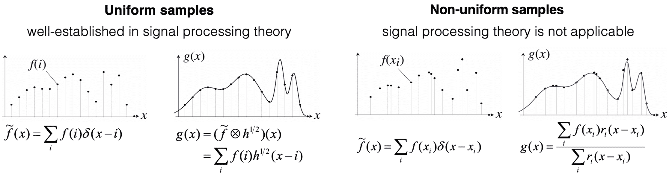
The continuous reconstruction of uniformly sampled functions or signals $\tilde{f}(x) = \sum_{i = 1}^n f(i) \delta(x - i)$ from the original function $f$ is well understood and described by signal processing theory, which is achieved by convolving the sampled signal with a reconstruction filter $h$. That is, the reconstructed signal $g$ can be obtained by $g(x) = (\tilde{f} \otimes h^{1/2}) (x)$ or equivalently $\sum_{i=1}^n f(i) h^{1/2} (x-i)$.

However, signal processing theory is not applicable to nonuniform samples and non-trivial in nonuniform samples. In this case, we can reconstruct a continuous signal g by building a weighted sum of reconstruction kernel $r$, akin to the uniform case: $g(x) = \sum_{i=1}^n f(x_i) r_i (x - x_i) / \sum_{j=1}^n r_j (x - x_j)$.

$\mathbf{Fig\ 7.}$ Continuous reconstruction in signal processing theory. (source: Matthias Zwicker)

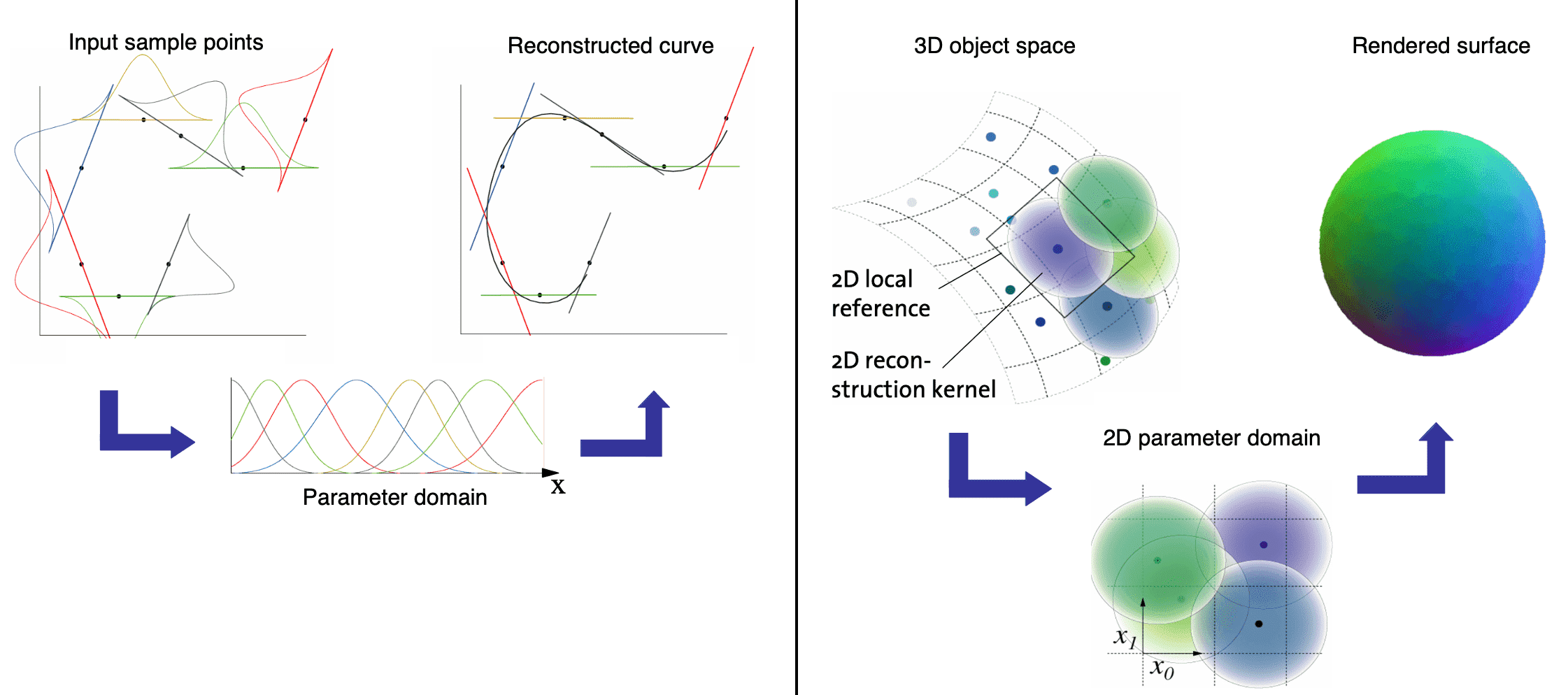
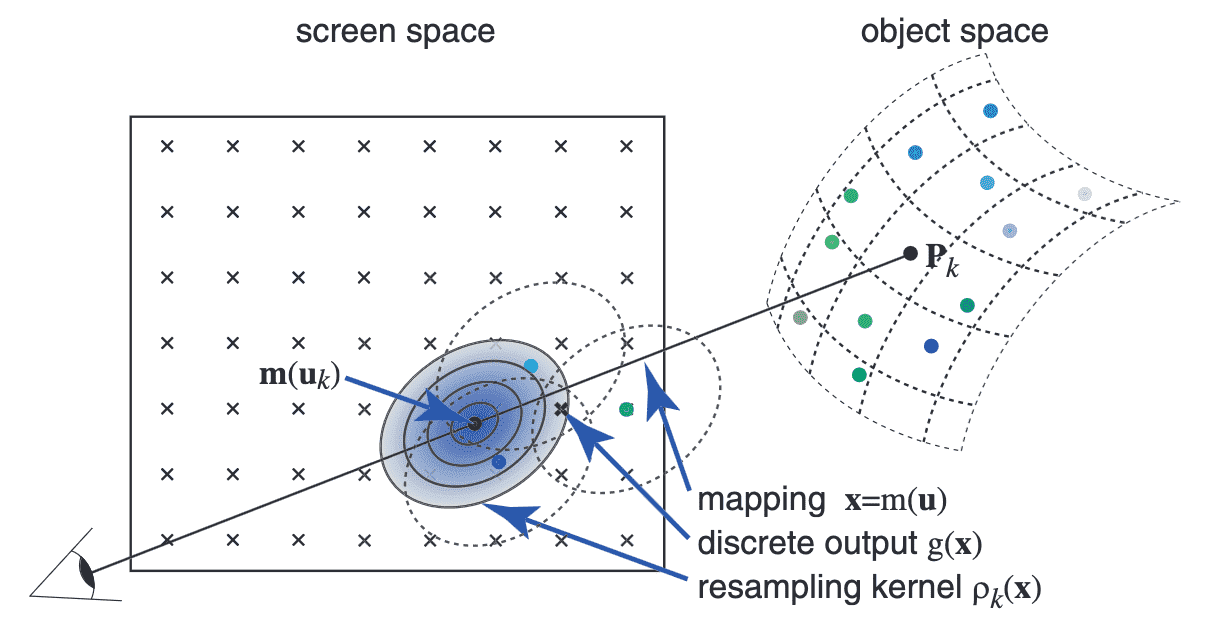
Intuitively, surfaces are interpreted as lower dimensional signals in a higher dimensional space. Through the discrete sampled points on the 3D object space, each point encapsulating representations of continuous texture functions (counterpart of reconstruction kernel) on its local coordinates, surface splatting aims to reconstruct a continuous surface on the 2D image space. Reconstruction is performed by computing the weighted sum of reconstruction kernels in image space.

$\mathbf{Fig\ 8.}$ Equivalence between parameterized signal reconstruction and surface splatting (source: Matthias Zwicker)

Moreover, to avoid aliasing artifacts, the surface splatting adopts the concept of resampling with prefiltering, which has been introduced to computer graphics by Paul Heckbert in 1989 in the context of texture filtering and image warping. Resampling includes the following steps:

1. A continuous signal is reconstructed in source space (counterpart of parameter space).
2. The continuous signal is then warped to destination space (counterpart of screen space).
3. A prefilter is applied to remove high frequencies from the warped signal, i.e., to band-limit the signal.
4. The band-limited signal is sampled at the new sampling grid in destination space, avoiding any aliasing artifacts.

2D Parameterization of Surface Texture

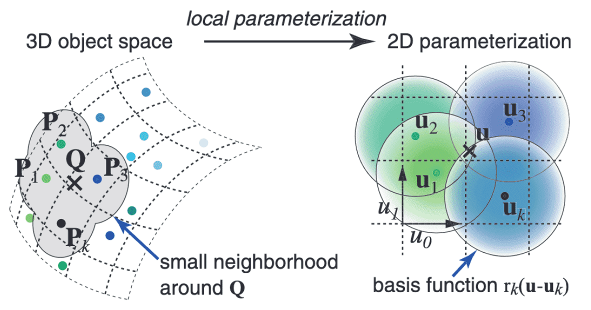
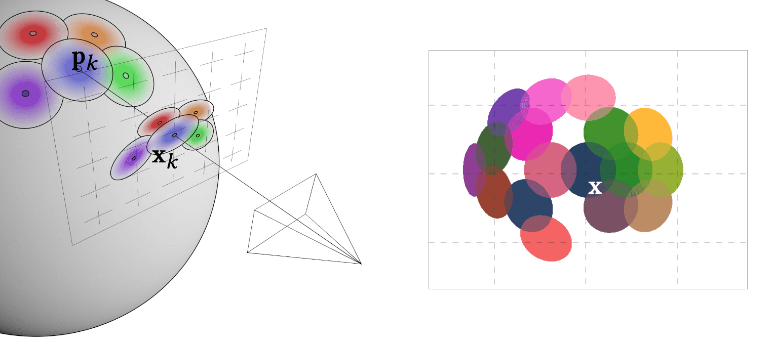
Let point-sampled surfaces be a set of irregularly spaced points ${ \mathbf{p}_k }$ in three-dimensional object space without connectivity. A point $\mathbf{p}_k$ has the corresponding position and surface normal, each associated with a basis function $r_k$ and coefficients $w_k^r$, $w_k^g$, $w_k^b$ for color channels. But without loss of generality, we proceed with the discussion using a single channel $w_k$. Since the 3D points are usually positioned irregularly, we simply adopt a weighted sum of radially symmetric basis functions. Given a point $\mathbf{q}$ on the surface with local coordinates $\mathbf{u}$ (i.e. coordinates in the local parametrization), the value of the continuous texture function is expressed as

\[f_c (\mathbf{u}) = \sum_{k \in \mathbb{N}} w_k r_k (\mathbf{u} - \mathbf{u}_k)\]

where $\mathbf{u}_k$ are the local coordinates of the point $\mathbf{p}_k$.

$\mathbf{Fig\ 9.}$ Defining a texture function on the surface of a point-based object. (source: Zwicker et al. SIGGRAPH 2001)

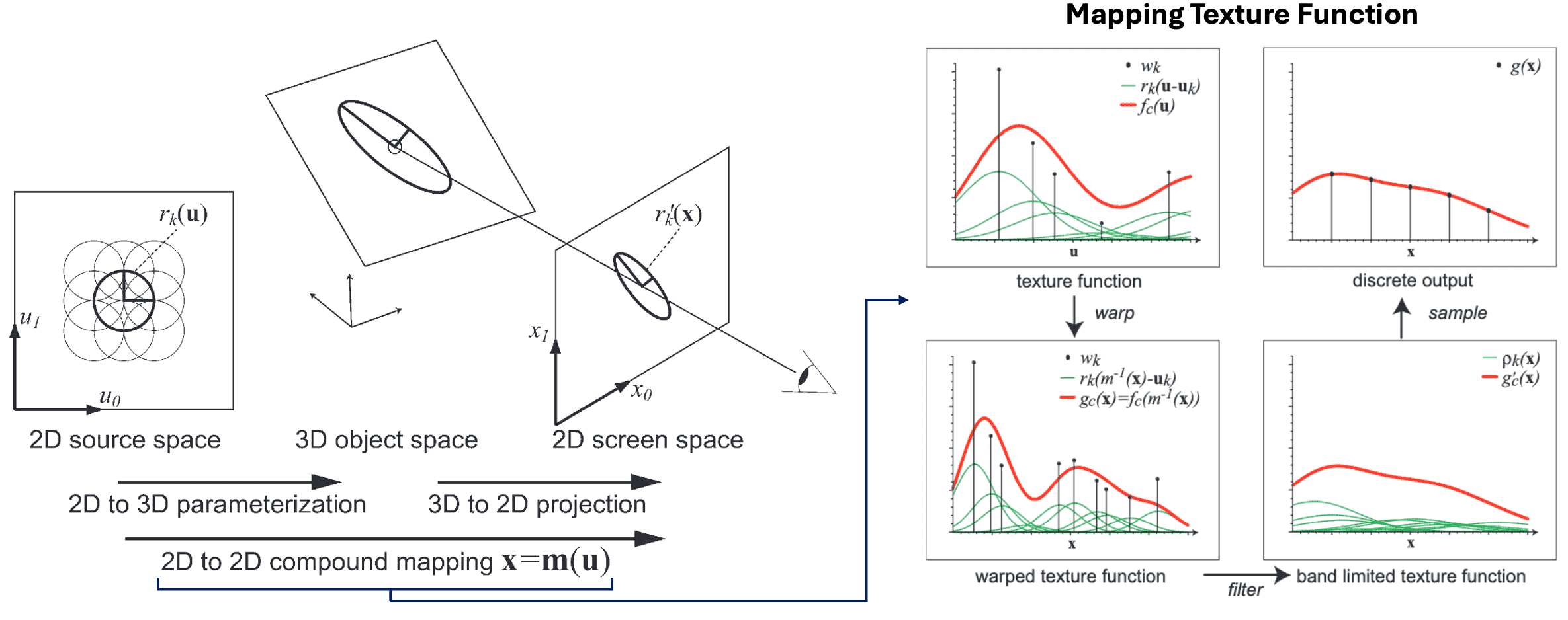
Mapping Texture to Screen

With this model at hand, we can view the task of rendering point-based objects as a concatenation of warping, filtering, and sampling the continuous texture function, as shown in $\mathbf{Fig\ 11}$. We denote the mapping from 2D parameterization space to 2D screen space by $\mathbf{x} = \mathbf{m}(\mathbf{u})$. Then, rendering involves these three steps:

1. Warping to screen space
   $$ g_c (\mathbf{x}) = (f_c \circ \mathbf{m}^{-1}) (\mathbf{x}) $$
2. Filtering
   To anti-aliasing, band-limit the screen space signal, to prevent exceeding Nyquist criterion, using a pre-filter $h$ ('pre' means prior to discretizing for display), resulting in the continuous output function $$ g_c (\mathbf{x}) = g_c (\mathbf{x}) \otimes h(\mathbf{x}) = \int_{\mathbb{R}^2} g_c (\xi) h(\mathbf{x} - \xi) \mathrm{d} \xi $$ where $\otimes$ denotes convolution. An explicit expression for $g_c (\mathbf{x})$ can be derived as follows: $$ \begin{aligned} g_c(\mathbf{x}) & =\int_{\mathbb{R}^2} h(\mathbf{x}-\xi) \sum_{k \in \mathbb{N}} w_k r_k\left(\mathbf{m}^{-1}(\xi)-\mathbf{u}_k\right) \mathrm{d} \xi \\ & =\sum_{k \in \mathbb{N}} w_k \rho_k(\mathbf{x}) \\ \text { where } & \rho_k(\mathbf{x})=\int_{\mathbb{R}^2} h(\mathbf{x}-\xi) r_k\left(\mathbf{m}^{-1}(\xi)-\mathbf{u}_k\right) \mathrm{d} \xi \end{aligned} $$ Here, a warped and filtered basis function $\rho_k (\mathbf{x})$ is termed a resampling kernel. This equation states that we can first warp and filter each basis function $r_k$ individually to construct the resampling kernels $\rho_k$ and then sum up the contributions of these kernels in screen space. The act of warping the basic function in this context, as mentioned in previous sections, is aligned with the act of projecting a surfel to screen-space. Hence, the authors coined this approach as surface splatting:
   
   

   

   $\mathbf{Fig\ 10.}$ Rendering by Surface splatting (source: Zwicker et al. SIGGRAPH 2001)
   
   In order to simplify the integral for $\rho_k$, we define the affine approximation $\mathbf{m}_{\mathbf{u}_k}$ of the object-to-screen mapping around point $\mathbf{u}_k$: $$ \begin{gathered} \mathbf{m}_{\mathbf{u}_{\mathbf{k}}}(\mathbf{u})=\mathbf{x}_{\mathbf{k}}+\mathbf{J}_{\mathbf{u}_{\mathbf{k}}} \cdot\left(\mathbf{u}-\mathbf{u}_{\mathbf{k}}\right) \\ \text{ where } \mathbf{x}_{\mathbf{k}}=\mathbf{m}\left(\mathbf{u}_{\mathbf{k}}\right) \text{ and the Jacobian } \left. \mathbf{J}_{\mathbf{u}_{\mathbf{k}}}=\frac{\partial \mathbf{m}}{\partial \mathbf{u}} \right\vert_{\mathbf{u} = \mathbf{u}_{\mathbf{k}}} \end{gathered} $$ Then, $\rho_k$ reduces to $$ \begin{aligned} \rho_k(\mathbf{x}) & =\int_{\mathbb{R}^2} h\left(\mathbf{x}-\mathbf{m}_{\mathbf{u}_k}\left(\mathbf{u}_k\right)-\xi\right) r_k^{\prime}(\xi) \mathrm{d} \xi \\ & =\left(r_k^{\prime} \otimes h\right)\left(\mathbf{x}-\mathbf{m}_{\mathbf{u}_k}\left(\mathbf{u}_k\right)\right) \end{aligned} $$ where $r_k^\prime (\mathbf{x}) = r_k (\mathbf{J}_{\mathbf{u}_{\mathbf{k}}}^{-1} \mathbf{x})$ denotes a warped basis function. Now, just omit the subscript $\mathbf{u}_k$ for $\mathbf{m}$ and $\mathbf{J}$ for brevity.
3. Discretization sampling
   Sample the continuous output function by multiplying it with an impulse train $i$ to produce the discrete output: $$ g(\mathbf{x}) = g_c^\prime (\mathbf{x}) i (\mathbf{x}). $$

$\mathbf{Fig\ 11.}$ Mapping a surface function from parameter space to screen space. (source: Zwicker et al. SIGGRAPH 2001)

EWA framework

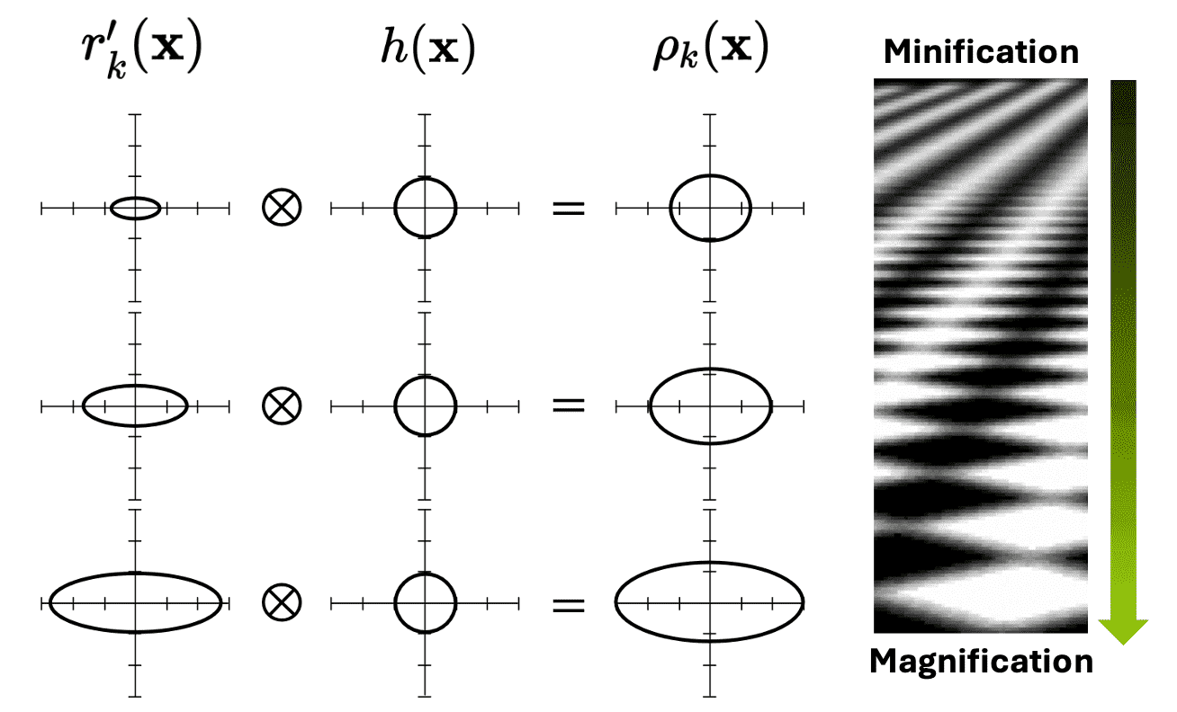
Then, how shall we designate $r_k$ and $h$? The original paper of surface splatting selected the EWA (Elliptical Weighted Average) framework; choosing 2D elliptical Gaussians $G$ both for the basis functions and filter:

\[G(\mathbf{x}; \mathbf{p}, \mathbf{V}) = \frac{1}{2\pi \lvert \mathbf{V} \rvert^{\frac{1}{2}}} e^{-\frac{1}{2} (\mathbf{x} - \mathbf{p})^\top \mathbf{V}^{-1} (\mathbf{x} - \mathbf{p})} \text{ where } \mathbf{p} \in \mathbb{R}^2, \mathbf{V} \in \mathbb{R}^{2 \times 2}\]

That is, we set $r_k(\mathbf{x}) = G(\mathbf{x}; \mathbf{0}, V) = G(\mathbf{x}; \mathbf{V}_k^r)$ and $h(\mathbf{x}) = G(\mathbf{x}; \mathbf{V}^h)$ (typically, we set $\mathbf{V}^h = \mathbf{I}$). The adoption of Gaussians is advantageous to us, as the resampling kernel can be expressed in a closed form as a single elliptical Gaussian again: the warped basis function $r_k^\prime$ and the resampling kernel $\rho_k$ are given by

\[\begin{aligned} r_k^\prime (\mathbf{x}) & = r (\mathbf{J}^{-1} \mathbf{x}) = \frac{1}{\vert \mathbf{J}^{-1}\vert} G(\mathbf{x}; \mathbf{J} \mathbf{V}_{k}^r \mathbf{J}^\top) \\ \rho_k(\mathbf{x}) & =\left(r_k^{\prime} \otimes h\right)\left(\mathbf{x}-\mathbf{m}\left(\mathbf{u}_k\right)\right) \\ & =\frac{1}{\left|\mathbf{J}^{-1}\right|}\left(G_{\mathbf{J V}_k^r \mathbf{J}^\top} \otimes G_{\mathbf{I}}\right)\left(\mathbf{x}-\mathbf{m}\left(\mathbf{u}_k\right)\right) \\ & =\frac{1}{\left|\mathbf{J}^{-1}\right|} G\left(\mathbf{x}-\mathbf{m}\left(\mathbf{u}_k\right); \mathbf{J V}_k^r \mathbf{J}^\top+\mathbf{I}\right) \end{aligned}\]

Hence, the continuous output function $g_c$ is given by

\[g_c (\mathbf{x}) = \sum_{k \in \mathbb{N}} w_k \frac{1}{\left|\mathbf{J}^{-1}\right|} G\left(\mathbf{x}-\mathbf{m}\left(\mathbf{u}_k\right); \mathbf{J V}_k^r \mathbf{J}^\top+\mathbf{I}\right)\]

The influence of Gaussian resampling kernels on the splat shape can be visualized as $\mathbf{Fig\ 12}$ and can be comprehended intuitively. EWA splatting employing elliptical Gaussian provides a smooth transition from minification to magnification. During minification, the warped basis function $r_k^\prime$ (i.e. the projected surfel) is notably small, and thus the prefilter $h$ is dominant. Consequently, the low-pass filter blurs the reconstruction kernel and removes its high frequencies. Conversely, for magnification, the size of $h$ is minute compared to $r_k^\prime$ and does not affect the splat shape significantly. It thus avoids unnecessary blurrying of the output image.

$\mathbf{Fig\ 12.}$ The effects of Gaussian resampling kernels (source: Matthias Zwicker)

EWA Volume Splatting

The discussion of (EWA) surface splatting can be directly extended to the point-based volume rendering. The volume rendering version of EWA surface splatting is referred to as EWA volume splatting, which is also proposed by Zwicker et al. VIS ‘01, the same authors of surface splatting in the same year.

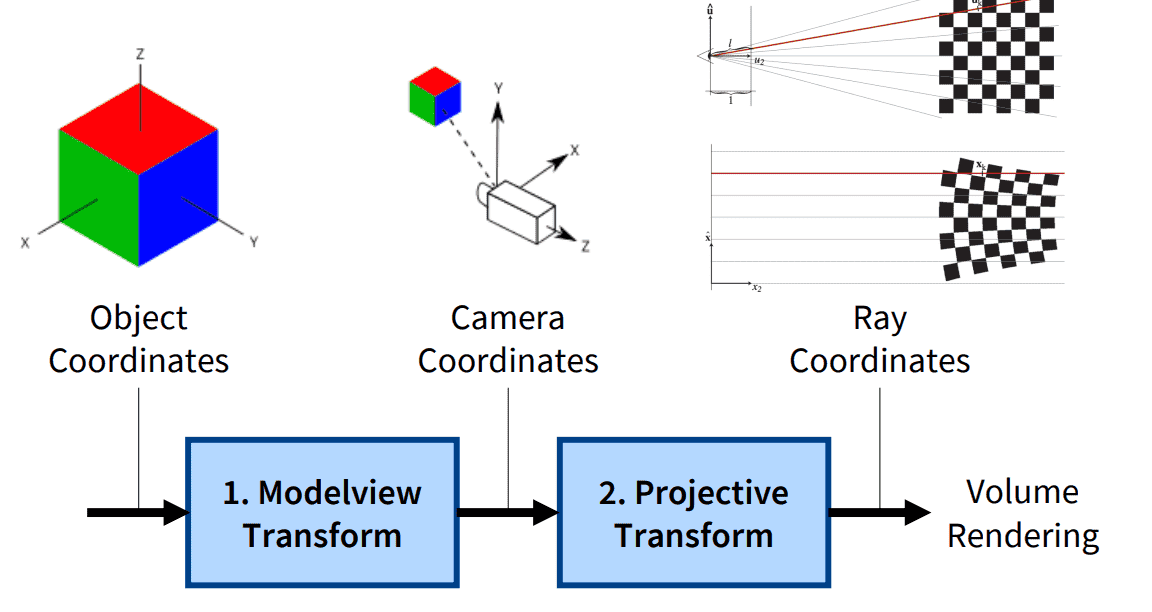
Volume Rendering Pipeline

Volume splatting is categorized into the forward mapping volume rendering that map the data onto the image plane, while the backward mapping volume rendering shoots rays through pixels on the image plane into the volume data. And mapping the volume data onto the image plane involves a sequence of intermediate steps where the data is transformed to different coordinate systems as traditional rasterization system. Here are the notations for coordinate systems in this post:

• $\mathbf{x}$: Object coordinates
• $\mathbf{x}^\prime = f(\mathbf{x})$: Camera coordinates
• $\mathbf{x}^{\prime \prime} = g(\mathbf{x}^\prime)$: Ray coordinates

$\mathbf{Fig\ 13.}$ The volume rendering pipeline (source: KEA SIGMA DELTA and Zwicker et al. 2001)

To rendering the volumetric object with volume rendering, the volume (3D) splats are necessitated instead of surface (2D) splats. Similar to EWA surface splat, each EWA volume splat is defined with the following attributes including parameters for elliptical Gaussian kernel but 3D:

• $\sigma$: opacity
• $\mathbf{c}$: color (can be extended view-dependent color, i.e. radiance)
• $\mathbf{p} \in \mathbb{R}^3$: center point
• $\mathbf{V} \in \mathbb{R}^{3 \times 3}$: covariance matrix that is symmetric, positive definite

Be aware that the parameters for Gaussian are define in the object coordinate system. Hence, we also need to

Model-View Transform

The reconstruction kernels are initially given in object space, and must be transformed to camera coordinates. Recall that this model-view transformation is defined by affine transformation $f$ with linear transformation $\mathbf{W}$ and the translation $\mathbf{t}$:

\[\begin{aligned} \mathbf{x}^\prime & = f(\mathbf{x}) = \mathbf{W} \mathbf{x} + \mathbf{t} \\ \mathbf{x} & = f^{-1} (\mathbf{x}) = \mathbf{W}^{-1} (\mathbf{x}^\prime - \mathbf{t}) \end{aligned}\]

Then, the Gaussian reconstruction kernel is transformed as follows:

\[\begin{aligned} & G(\mathbf{x} ; \mathbf{p}, \mathbf{V})=\frac{1}{(2 \pi)^{\frac{3}{2}\vert \mathbf{V} \vert^{\frac{1}{2}}}} e^{-\frac{1}{2}(\mathbf{x}-\mathbf{p})^\top \mathbf{V}^{-1}(\mathbf{x}-\mathbf{p})} \\ & =\frac{1}{(2 \pi)^{\frac{3}{2}}\vert \mathbf{V} \vert^{\frac{1}{2}}} e^{-\frac{1}{2}\left\{\mathbf{W}^{-1}\left(\mathbf{x}^{\prime}-\mathbf{t}\right)-\mathbf{W}^{-1}\left(\mathbf{p}^{\prime}-\mathbf{t}\right)\right\}^\top \mathbf{V}^{-1}\left\{W^{-1}\left(\mathbf{x}^{\prime}-\mathbf{t}\right)-W^{-1}\left(\mathbf{p}^{\prime}-\mathbf{t}\right)\right\}} \\ & =\frac{1}{(2 \pi)^{\frac{3}{2}}\vert \mathbf{V}\vert ^{\frac{1}{2}}} e^{-\frac{1}{2}\left\{\mathbf{W}^{-1}\left(\mathbf{x}^{\prime}-\mathbf{p}^{\prime}\right)\right\}^\top \mathbf{V}^{-1}\left\{\mathbf{W}^{-1}\left(\mathbf{x}^{\prime}-\mathbf{p}^{\prime}\right)\right\}}=\frac{1}{(2 \pi)^{\frac{3}{2}}\vert \mathbf{V}\vert ^{\frac{1}{2}}} e^{-\frac{1}{2}\left(\mathbf{x}^{\prime}-\mathbf{p}^{\prime}\right)^\top \mathbf{W}^{-\mathrm{T}} \mathbf{V}^{-1} \mathbf{W}^{-1}\left(\mathbf{x}^{\prime}-\mathbf{p}^{\prime}\right)} \\ & =\frac{1}{(2 \pi)^{\frac{3}{2}}\vert \mathbf{V} \vert^{\frac{1}{2}}} e^{-\frac{1}{2}\left(\mathbf{x}^{\prime}-\mathbf{p}^{\prime}\right)^\top\left(\mathbf{V}^{\prime}\right)^{-1}\left(\mathbf{x}^{\prime}-\mathbf{p}^{\prime}\right)}=\frac{\vert \mathbf{W} \vert }{(2 \pi)^{\frac{3}{2}\left\vert \mathbf{V}^{\prime}\right\vert ^{\frac{1}{2}}}} e^{-\frac{1}{2}\left(\mathbf{x}^{\prime}-\mathbf{p}^{\prime}\right)^\top\left(\mathbf{V}^{\prime}\right)^{-1}\left(\mathbf{x}^{\prime}-\mathbf{p}^{\prime}\right)} \\ & =\vert \mathbf{W} \vert G\left(\mathbf{x}^{\prime} ; \mathbf{p}^{\prime}, \mathbf{V}^{\prime}\right) \end{aligned}\]

where the transformed Gaussian parameters are given by

\[\begin{aligned} \mathbf{p}^\prime & = \mathbf{W}\mathbf{p} + \mathbf{t} \\ \mathbf{V}^\prime & = \mathbf{W}\mathbf{V}\mathbf{W}^\top \end{aligned}\]

Projective Transform

Ray space is a non-cartesian coordinate system that enables an easy formulation of the volume rendering equation. In ray space, the viewing rays are parallel to a coordinate axis, facilitating analytical integration of the volume function. We denote a point in ray space by a column vector of three coordinates $\mathbf{x}^{\prime\prime} = (x_1^{\prime\prime}, x_2^{\prime\prime}, x_3^{\prime\prime})^\top$. The coordinates $(x_1^{\prime\prime}, x_2^{\prime\prime})$ specify a point on the projection plane; that is, the origin of the corresponding viewing ray. And the third coordinate $x_3^{\prime\prime}$ specifies the Euclidean distance from the center of projection to a point on the viewing ray.

Setting the $z$-coordinate of projection plane to be $z = 1$, the projective transformation converts camera coordinates to ray coordinates using simple triangle similarity as illustrated in the $\mathbf{Fig\ 14}$.

$\mathbf{Fig\ 14.}$ Transforming the volume from camera to ray space. Top: camera space. Bottom: ray space. (source: Zwicker et al. 2001)

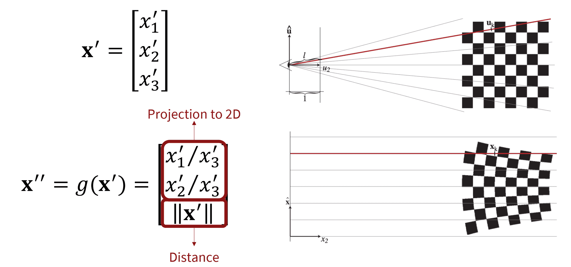
Unfortunately, these mappings are not affine, so we cannot obtain the closed form of projected Gaussian kernel simply on the ray space. To address this issue, EWA volume splatting locally approximates the projective transformation with an affine transformation at each splat, of which Gaussian parameters are $\mathbf{p}_i^\prime$ and $\mathbf{V}_i^\prime$ on the camera space, using the first-order Taylor expansion:

\[\begin{aligned} g(\mathbf{x}^\prime) & \approx g(\mathbf{p}_i^\prime) + \mathbf{J}_{\mathbf{p}_i^\prime} (\mathbf{x}^\prime - \mathbf{p}_i^\prime) \\ & = \mathbf{J}_{\mathbf{p}_i^\prime} \mathbf{x}^\prime + (g(\mathbf{p}_i^\prime) - \mathbf{J}_{\mathbf{p}_i^\prime} \mathbf{p}_i^\prime) \end{aligned}\]

where the Jacobian \(\mathbf{J}_{\mathbf{p}_i^\prime} = \frac{\partial g(\mathbf{x}^\prime)}{\partial \mathbf{x}^\prime} \vert_{\mathbf{x}^\prime = \mathbf{p}_i^\prime}\) is given by

\[\mathbf{J} =\left[\begin{array}{ccc} 1 / x_3^{\prime} & 0 & -x_1^{\prime} /\left(x_3^{\prime}\right)^2 \\ 0 & 1 / x_3^{\prime} & -x_2^{\prime} /\left(x_3^{\prime}\right)^2 \\ x_1^{\prime} /\left\|\mathbf{x}^{\prime}\right\| & x_2^{\prime} /\left\|\mathbf{x}^{\prime}\right\| & x_3^{\prime} /\left\|\mathbf{x}^{\prime}\right\| \end{array}\right]\]

Thus, analogous to the previous section, the transformed Gaussian kernel into ray space is derived as

\[G (g^{-1} (\mathbf{x}^{\prime\prime}); \mathbf{p}_i^\prime, \mathbf{V}_i^\prime) = \vert \mathbf{J}_{\mathbf{p}_i^\prime} \rvert G (\mathbf{x}^{\prime\prime}; \mathbf{p}_i^{\prime\prime}, \mathbf{V}_i^{\prime\prime})\]

with transformed Gaussian parameters

\[\begin{aligned} \mathbf{p}_i^{\prime\prime} & = g(\mathbf{p}_i^{\prime}) \\ \mathbf{V}_i^{\prime\prime} & = \mathbf{J}_{\mathbf{p}_i^\prime} \mathbf{V}_i^\prime \mathbf{J}_{\mathbf{p}_i^\prime}^\top \end{aligned}\]

Volume Rendering

For each ray $\mathbf{r}$ of the 2D pixel origin $(x, y)$ coordinates in the ray coordinate system $\mathbf{x}^{\prime\prime}$, recall that we compute the following volume rendering equation:

\[\begin{aligned} C (\mathbf{r}) & = \int_0^{z_\max} \mathbf{c}(z) \sigma (z) \mathcal{T}(z) \mathrm{d}z \\ & = \int_0^{z_\max} \mathbf{c}(z) \sigma (z) \exp \left( - \int_0^z \sigma(t) \mathrm{d}t \right) \mathrm{d}z \\ \end{aligned}\]

where $z$ denotes the distance alongthe ray. Analogous to surface splatting, we define the opacity as the weighted sum of elliptical Gaussian kernels of volume splats, keeping in mind that $\mathbf{p}_i$ and $\mathbf{V}_i$ are defined in the object coordinate system:

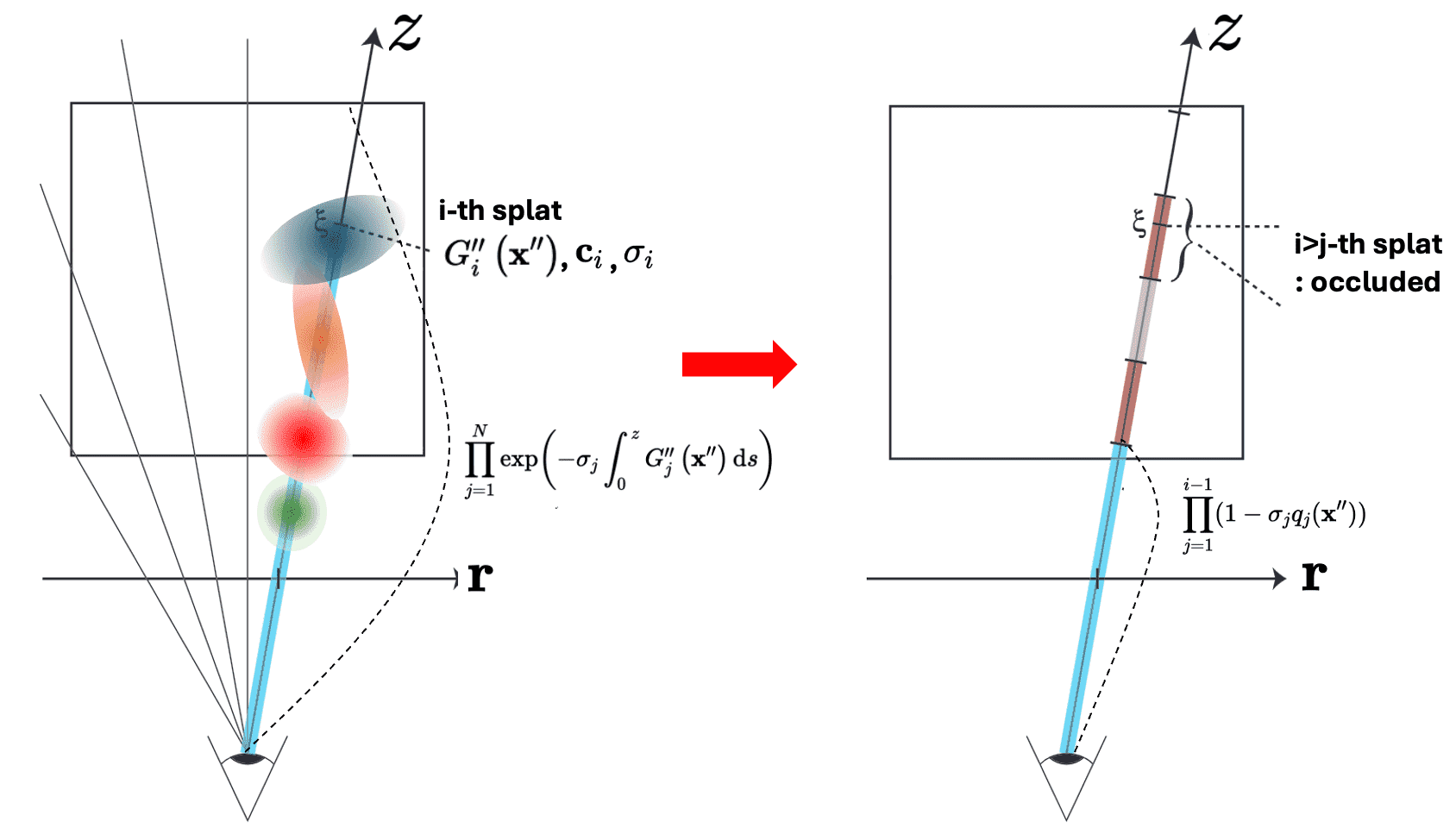
\[\sigma (z) = \sigma(\mathbf{x}^{\prime \prime}) = \sum_{i = 1}^N \sigma_i G (f^{-1} (g^{-1} (\mathbf{x}^{\prime\prime})); \mathbf{p}_i, \mathbf{V}_i) = \sum_{i = 1}^N \sigma_i G_i^{\prime \prime} (\mathbf{x}^{\prime\prime})\]

For brevity, let $G (f^{-1} (g^{-1} (\mathbf{x}^{\prime\prime})); \mathbf{p}_i, \mathbf{V}_i) = G_i^{\prime \prime} (\mathbf{x}^{\prime\prime})$. Assuming that the emission term $\mathbf{c}(z)$ is constant in the support of each reconstruction kernel along a ray, we can also write

\[\mathbf{c}(z) \sigma(z) = \sum_{i=1}^N \mathbf{c}_i \sigma_i G_i^{\prime \prime} (\mathbf{x}^{\prime\prime})\]

Then the color of ray $C (\mathbf{r})$ is rewritten as follows:

\[\begin{aligned} & C(\mathbf{r})=\int_0^{z_{\max }} \mathbf{c}(z) \sigma(z) \exp \left(-\int_0^t \sigma(z) \mathrm{d}s\right) \mathrm{d} z \\ & =\int_0^{z_{\max }}\left(\sum_{i=1}^N \mathbf{c}_i \sigma_i G_i^{\prime \prime}\left(\mathbf{x}^{\prime \prime}\right)\right) \exp \left(-\int_0^z\left(\sum_{j=1}^N \sigma_j G_j^{\prime \prime}\left(\mathbf{x}^{\prime \prime}\right)\right) \mathrm{d}s\right) \mathrm{d} z \\ & \quad=\sum_{i=1}^N \mathbf{c}_i \sigma_i\left(\int_0^{z_{\max }} G_i^{\prime \prime}\left(\mathbf{x}^{\prime \prime}\right) \prod_{j=1}^N \exp \left(-\sigma_j \int_0^z G_j^{\prime \prime}\left(\mathbf{x}^{\prime \prime}\right) \mathrm{d}s\right) \mathrm{d} z\right) \end{aligned}\]

To compute this function numerically, splatting algorithms introduce additional simplifying assumptions. It assumes that the local support of reconstruction kernel $G$ (recall that the Gaussian’s value is concentrated around its center) is non-overlapping. Therefore, self-occlusion occurs, rendering further splats occluded by closer splat; $G_{j > i}^{\prime\prime} (\mathbf{x}^{\prime\prime}) = 0$ if $G_i^{\prime\prime} (\mathbf{x}^{\prime\prime}) > 0$ as shown in $\mathbf{Fig\ 15.}$

$\mathbf{Fig\ 15.}$ Approximations of self-occlusion in volume splatting algorithms (source: Zwicker et al. 2001)

With Taylor approximation of exponential function $e^x \approx 1 - x$, the equation finally reduces to

\[\begin{aligned} C(\mathbf{r}) & = \sum_{i=1}^N \mathbf{c}_i \sigma_i\left(\int_0^{z_{\max }} G_i^{\prime \prime}\left(\mathbf{x}^{\prime \prime}\right) \prod_{j=1}^N \exp \left(-\sigma_j \int_0^z G_j^{\prime \prime}\left(\mathbf{x}^{\prime \prime}\right) \mathrm{d}s\right) \mathrm{d} z\right) \\ & = \sum_{i=1}^N \mathbf{c}_i \sigma_i q_i (\mathbf{x}^{\prime\prime}) \prod_{j=1}^{i - 1} (1 - \sigma_{j} q_j (\mathbf{x}^{\prime\prime})) \end{aligned}\]

where $q_i (\mathbf{x}^{\prime\prime}) = \int_0^{z_\max} G_i^{\prime\prime} (\mathbf{x}^{\prime\prime}) \mathrm{d}z$ denotes an integrated reconstruction kernel. And $q_i$ can be computed by a 1D integral along the axis, derived from the transformations of Gaussian kernels we’ve discussed in the previous sections:

\[\begin{aligned} q_i (\mathbf{x}^{\prime\prime}) & = \int_0^{z_\max} G (f^{-1}(g^{-1}(\mathbf{x}^{\prime\prime})), \mathbf{p}_i, \mathbf{V}_i) \; \mathrm{d}z \\ & = \lvert \mathbf{J}_{\mathbf{p}_i^{\prime\prime}} \rvert \lvert \mathbf{W} \rvert \int_0^{z_\max} G (\mathbf{x}^{\prime\prime}, \mathbf{p}_i^{\prime\prime}, \mathbf{V}_i^{\prime\prime}) \; \mathrm{d}z \end{aligned}\]

Differentiable Surface Splatting (DSS)

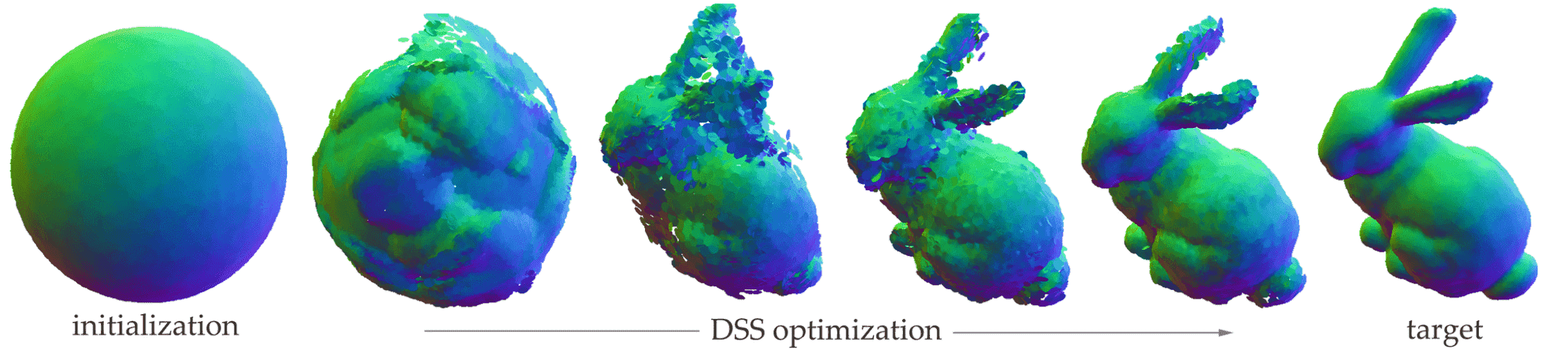
A notable recent advancement in splatting is the differentiable surface splatting (DSS). This approach elevates the simple rasterization pipeline of surface splatting to a differentiable rendering techniques, marking it as the first high-fidelity point-based differentiable renderer.

$\mathbf{Fig\ 16.}$ DSS successfully deforms a sphere to a target bunny model, capturing both large scale and fine-scale structure. (source: Yifan et al. 2019)

Forward pass

The forward pass of DSS closely follows the screen space EWA filtering of surface splatting. However, to build a differentiable renderer, it is worth noting two sources of discontinuity are introduced to rendering. The authors reformulated resampling kernel \(\bar{\rho}_k (\mathbf{x}) = \frac{1}{\left\vert\mathbf{J}^{-1}\right\vert} G\left(\mathbf{x}-\mathbf{m}\left(\mathbf{u}_k\right); \mathbf{J V}_k^r \mathbf{J}^\top+\mathbf{I}\right)\) as \(\rho_k (\mathbf{x}) = h_{\mathbf{x}} (\mathbf{p}_k) \bar{\rho}_k (\mathbf{x})\) where

\[h_\mathbf{x} (\mathbf{p}_k) = \begin{cases} 0 & \quad \text{ if } \frac{1}{2} \mathbf{x}^\top (\mathbf{J V}_k^r \mathbf{J}^\top+\mathbf{I}) \mathbf{x} > C \\ 0 & \quad \text{ if } \mathbf{p}_k \text{ is invisible at } \mathbf{x} \\ 1 & \quad \text{ otherwise } \end{cases}\]

1. For computational reasons, the authors truncate the elliptical Gaussians to a limited support in the image plane for all $\mathbf{x}$ outside a cutoff radius $C$: $$ \frac{1}{2} \mathbf{x}^\top (\mathbf{J V}_k^r \mathbf{J}^\top+\mathbf{I}) \mathbf{x} > C $$
2. Set the Gaussian weights for occluded points to zero.

Hence, the final pixel value at $\mathbf{x}$, denoted as $\mathbb{I}_{\mathbf{x}}$, is simply the sum of all filtered point attributes \(\{ w_k \}_{k=1}^N\) evaluated at the center of pixels.

$\mathbf{Fig\ 17.}$ Illustration of forward splatting (source: Yifan et al. 2019)

Backward pass

For the rendered image $\mathbb{I}$ by differentiable render $\mathcal{R}$ with the scene-specific paraemter $\theta$, i.e. $\mathbb{I} = \mathcal{R} (\theta)$, we necessitate the gradient $\frac{\mathrm{d} \mathbb{I}}{\mathrm{d} \theta}$ and aim to the solve an optimization problem

\[\theta^* = \underset{\theta}{\text{ arg min }} \mathcal{L} (\mathcal{R}(\theta), \mathbb{I}^*)\]

where $\mathcal{L}$ is the image loss and $\mathbb{I}^*$ is a reference image. The key to address the discontinuity of $\mathcal{R}$ is approximating gradients with regard to point coordinates $\mathbf{p}$ and normals $\mathbf{n}$, i.e. $\frac{\mathrm{d} \mathbb{I}}{\mathrm{d} \mathbf{p}}$ and $\frac{\mathrm{d} \mathbb{I}}{\mathrm{d} \mathbf{n}}$, since $\mathcal{R}$ is a discontinuous function due to occlusion events and edges thus these gradients are not defined everywhere.

The key observation of authors is that the discontinuity of $\mathcal{R}$ is encapsulated in the truncated Gaussian weights $\rho_k$, especially a discontinuous visibility term $h_\mathbf{x}$ whereas \(\bar{\rho}_k\) is the fully differentiable term. Writing a rendered image \(\mathbb{I}_{\mathbf{x}}\) as a function of $w_k$, \(\bar{\rho}_k\), and \(h_{\mathbf{x}}\), by chain rule:

\[\begin{aligned} \frac{\mathrm{d} \mathbb{I}_{\mathbf{x}}\left(w_k, \bar{\rho}_k, h_{\mathbf{x}}\right)}{\mathrm{d} \mathbf{n}_k} & = \frac{\partial \mathbb{I}_{\mathbf{x}}}{\partial w_k} \frac{\partial w_k}{\partial \mathbf{n}_k}+\frac{\partial \mathbb{I}_{\mathbf{x}}}{\partial \bar{\rho}_k} \frac{\partial \bar{\rho}_k}{\partial \mathbf{n}_k} + \frac{\partial \mathbb{I}_{\mathbf{x}}}{\partial h_{\mathbf{x}}} \frac{\partial h_{\mathbf{x}}}{\partial \mathbf{n}_k} \\ & = \frac{\partial \mathbb{I}_{\mathbf{x}}}{\partial w_k} \frac{\partial w_k}{\partial \mathbf{n}_k}+\frac{\partial \mathbb{I}_{\mathbf{x}}}{\partial \bar{\rho}_k} \frac{\partial \bar{\rho}_k}{\partial \mathbf{n}_k} \\ \frac{\mathrm{d} \mathbb{I}_{\mathbf{x}}\left(w_k, \bar{\rho}_k, h_{\mathbf{x}}\right)}{\mathrm{d} \mathbf{p}_k} & =\frac{\partial \mathbb{I}_{\mathbf{x}}}{\partial w_k} \frac{\partial w_k}{\partial \mathbf{p}_k}+\frac{\partial \mathbb{I}_{\mathbf{x}}}{\partial \bar{\rho}_k} \frac{\partial \bar{\rho}_k}{\partial \mathbf{p}_k}+\frac{\partial \mathbb{I}_{\mathbf{x}}}{\partial h_{\mathbf{x}}} \frac{\partial h_{\mathbf{x}}}{\partial \mathbf{p}_k} \end{aligned}\]

Here, the only non-differentiable term required to be approximated is \(\frac{\partial h_{\mathbf{x}}}{\partial \mathbf{p}_k}\), since it is undefined at the boundary of the ellipse. Approximating \(\phi_{\mathbf{x}} (\mathbf{p}_k) = \mathbb{I}_{\mathbf{x}} (h_{\mathbf{x}} (\mathbf{p}_k ))\) as a linear function defined by the change of point position \(\Delta \mathbf{p}_k\) and the pixel intensity \(\Delta \mathbb{I}_{\mathbf{x}}\) before and after the visibility change, we obtain the approximated gradient as follows:

\[\left.\frac{\mathrm{d} \Phi_\mathbf{x}}{\mathrm{d} \mathbf{p}_k}\right|_{\mathbf{p}_{k, 0}}= \begin{cases}\frac{\Delta \mathbb{I}_{\mathbf{x}}}{\left\|\Delta \mathbf{p}_k^{+}\right\|^2+\epsilon} \Delta \mathbf{p}_k^{+} & \mathbf{p}_k \text { invisible at } \mathbf{x} \\ \frac{\Delta \mathbb{I}_{\mathbf{x}}}{\left\|\Delta \mathbf{p}_k^{-}\right\|^2+\epsilon} \Delta \mathbf{p}_k^{-}+\frac{\Delta \mathbb{I}_{\mathbf{x}}}{\left\|\Delta \mathbf{p}_k^{+}\right\|+\epsilon} \Delta \mathbf{p}_k^{+} & \text {otherwise}\end{cases}\]

where \(\Delta \mathbf{p}_k^−\) and \(\Delta \mathbf{p}_k^+\) denote the point movement toward and away from $\mathbf{x}$, starting from the current position $\mathbf{p}_{k,0}$.

For understanding of the formula, first consider a simplified scenario where a single point only moves in 1D space. As shown in the following figure, $\phi_{\mathbf{x}}$ is generally discontinuous and zero almost everywhere except in a small region around $\mathbf{q}_\mathbf{x}$ where it is the coordinates of the pixel $\mathbf{x}$ back-projected to world coordinates.

$\mathbf{Fig\ 18.}$ An illustration of the artificial gradient in two 1D scenarios: the ellipse centered at $\mathbf{p}_{k, 0}$ is (a) invisible and (b) visible at pixel $\mathbf{x}$. (source: Yifan et al. 2019)

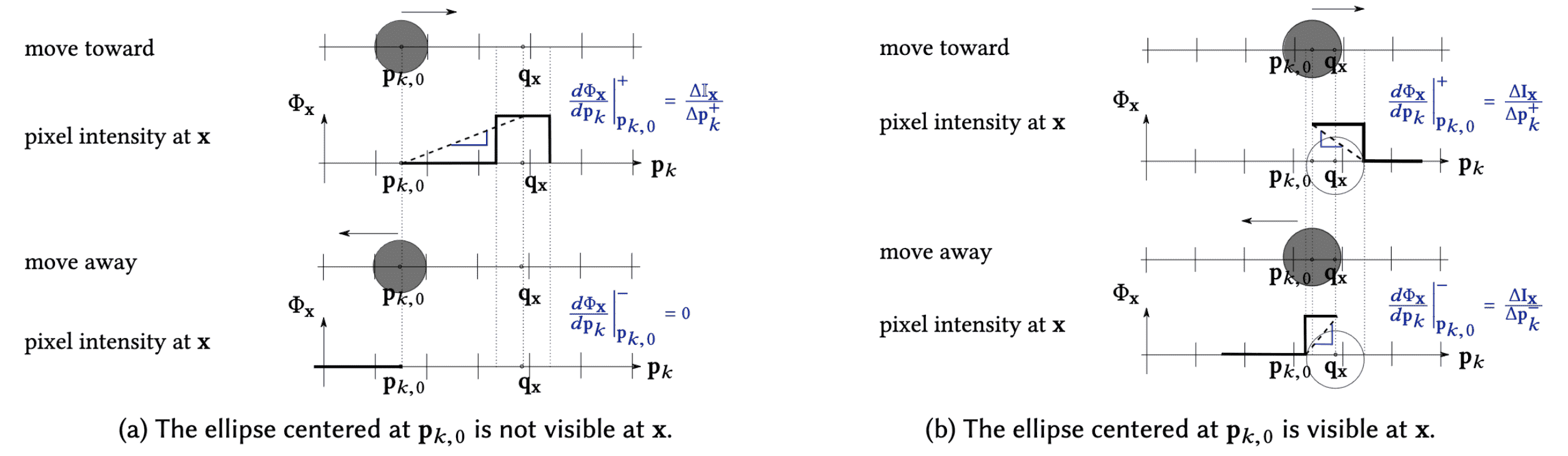
As \(\mathbf{p}_k\) approaches or recedes from \(\mathbf{q}_{\mathbf{x}}\), two distinct linear functions are obtained, with gradients \(\left.\frac{\mathrm{d} \Phi_\mathbf{x}}{\mathrm{d} \mathbf{p}_k}\right\vert_{\mathbf{p}_{k, 0}}^+\) and \(\left.\frac{\mathrm{d} \Phi_\mathbf{x}}{\mathrm{d} \mathbf{p}_k}\right\vert_{\mathbf{p}_{k, 0}}^-\), respectively. When $\mathbf{p}_k$ is invisible at $\mathbf{x}$, moving away will always yield gradient of $0$. Conversely, when \(\mathbf{p}_k\) is visible, we obtain two gradients but with opposite signs. And, to mitigate the risk of the gradient becoming excessively large when \(\mathbf{p}_k\) approaches \(\mathbf{q}_\mathbf{x}\), a small constant $\epsilon$ is further introduced into the denominator of gradient.

3D Gaussian Splatting (3DGS)

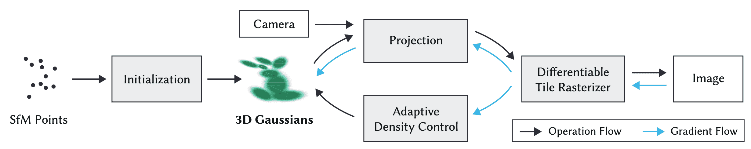
As EWA volume splatting, 3D Gaussian Splatting (3DGS) directly optimizes 3D Gaussian ellipsoids to which attributes like 3D position $P$, rotation $R$, scale $S$, opacity $\alpha$ and Spherical Harmonic (SH) coefficients representing view-dependent color are attached. It first initializes splats with the sparse points from SfM, updates the splats parameters with $L_1$ and SSIM loss through gradient descents along the end-to-end differentiable rendering pipeline.

$\mathbf{Fig\ 19.}$ Overview of 3D Gaussian Splatting (source: Kerbl et al. 2023)

View-dependent Color with SH

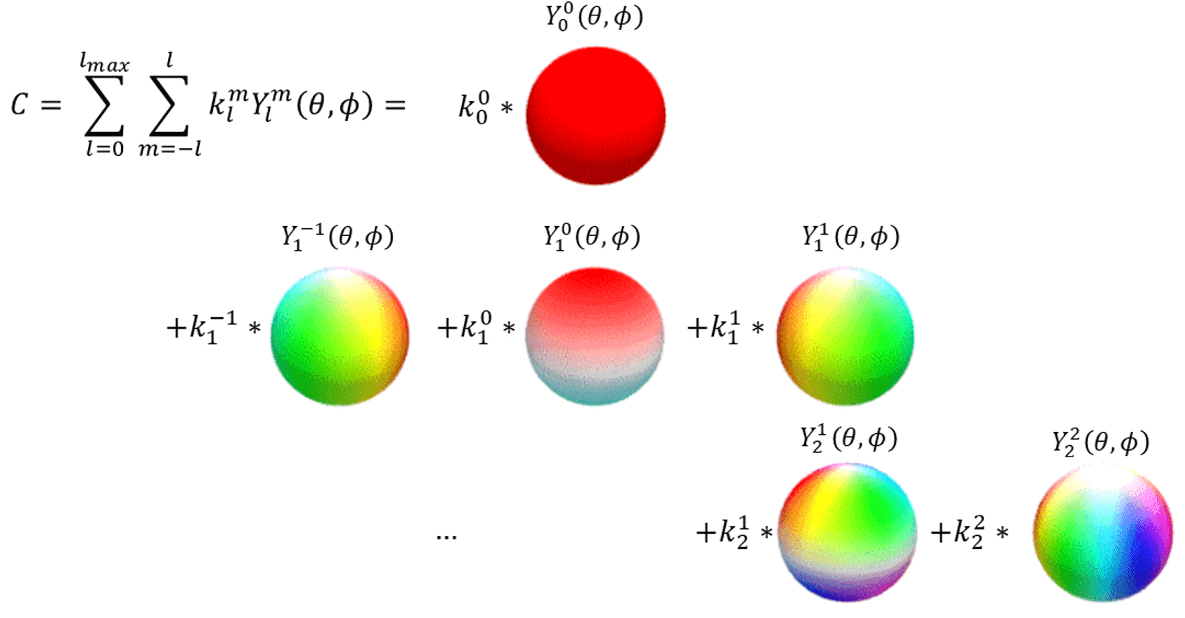
SH coefficients $c$represents a view-dependent color computed by spherical harmonics functions. Given any point on the sphere $(\theta, \phi)$, spherical harmonics function with parameters $(m, \ell)$, where $- \ell \leq m \leq \ell$, $Y_\ell^m (\theta, \phi)$ is defined as

\[Y_\ell^m(\theta, \phi)=\frac{(-1)^\ell}{2^\ell \ell!} \sqrt{\frac{(2 \ell+1)(\ell+m)!}{4 \pi(\ell-m)!}} e^{i m \phi}(\sin \theta)^{-m} \frac{\mathrm{d}^{\ell-m} (\sin \theta)^{2 \ell}}{\mathrm{d}(\cos \theta)^{\ell-m}}\]

Thus, SH functions are defined on the surface of a sphere and first introduced in spherical harmonic lighting of Green et al. SIGGRAPH 2003. Considering SH functions as orthogonal basis, it computes the SH coefficient $c$ of an arbitrary function $f$ as follows:

\[\begin{aligned} f(\theta, \phi) & =\sum_{\ell=0}^{\infty} \sum_{m=-\ell}^\ell f_{\ell}^m Y_\ell^m(\theta, \phi) \\ f_{\ell}^m & =\int_{\phi=0}^{2 \pi} \int_{\theta=0}^\pi f(\theta, \phi) {Y_\ell^m}^*(\theta, \phi) \sin \theta \; \mathrm{d} \theta \; \mathrm{d} \phi \end{aligned}\]

Substituting $f$ with the lighting function, color representation can be achieved through SH coefficients. And these coefficients can subsequently be converted from SH coefficients to obtain the desired color representation.

$\mathbf{Fig\ 20.}$ A process of obtaining a view-dependant color via SH coefficients (source: tistroy)

Optimizing 3D Gaussians

To directly optimize the parameters of 3D Gaussian splat, it’s imperative to ensure that the Gaussian covariance retains its physical meaning throughout the process of back-propagation. Recall that the projection of the covariance $\Sigma$ 3D Gaussian ellipsoids one 2D image from a viewpoint is given by

\[\Sigma^\prime = J W \Sigma W^\top J^\top\]

where $W$ is the viewing transformation matrix and $J$ is the Jacobian matrix for the projective transformation. To force the positive semi-definiteness constraint of covariance $\Sigma$ while back-propagation, 3DGS formulates $\Sigma$ as

\[\Sigma = RSS^\top R^\top\]

given corresponding scaling matrix $S$ and rotation matrix $R$, with corresponding quaternions $\mathbf{s}$ and $\mathbf{q}$ respectively. Then, all associated gradients for optimization have closed-form expressions, thereby circumventing the overhead due to automatic differentiation. By letting $U = JW$ and $M = RS$, i.e. $\Sigma^\prime = U \Sigma U^\top$ and $\Sigma = MM^\top$, we obtain

\[\begin{aligned} & \frac{\mathrm{d} \Sigma^\prime}{\mathrm{d} \mathbf{s}} = \frac{\mathrm{d} \Sigma^\prime}{\mathrm{d} \Sigma} \frac{\mathrm{d} \Sigma}{\mathrm{d} \mathbf{s}}, \; \frac{\mathrm{d} \Sigma^\prime}{\mathrm{d} \mathbf{q}} = \frac{\mathrm{d} \Sigma^\prime}{\mathrm{d} \Sigma} \frac{\mathrm{d} \Sigma}{\mathrm{d} \mathbf{q}} \\ & \frac{\partial \Sigma^\prime}{\partial \Sigma_{ij}} = \begin{bmatrix} U_{1,i} U_{1,j} & U_{1,i} U_{2,j} \\ U_{2,i} U_{1,j} & U_{2,i} U_{2,j} \end{bmatrix} \\ & \frac{\mathrm{d} \Sigma}{\mathrm{d} \mathbf{s}} = \frac{\mathrm{d} \Sigma}{\mathrm{d} M} \frac{\mathrm{d} M}{\mathrm{d} \mathbf{s}}, \; \frac{\mathrm{d} \Sigma}{\mathrm{d} \mathbf{q}} = \frac{\mathrm{d} \Sigma}{\mathrm{d} M} \frac{\mathrm{d} M}{\mathrm{d} \mathbf{q}} \\ & \frac{\mathrm{d} \Sigma}{\mathrm{d} M} = 2M^\top \\ & \frac{\partial M_{i,j}}{\partial \mathbf{s}_k} = \begin{cases} R_{i, k} & \quad \text{ if } j = k \\ 0 & \quad \text{ otherwise } \end{cases} \\ & \frac{\partial M}{\partial \mathbf{q}_r} = 2 \begin{bmatrix} 0 & -\mathbf{s}_y \mathbf{q}_k & \mathbf{s}_z \mathbf{q}_j \\ \mathbf{s}_x \mathbf{q}_k & 0 & -\mathbf{s}_z \mathbf{q}_i \\ -\mathbf{s}_x \mathbf{q}_j & \mathbf{s}_y \mathbf{q}_i & 0 \end{bmatrix}, \; \frac{\partial M}{\partial \mathbf{q}_i} =2 \begin{bmatrix} 0 & \mathbf{s}_y \mathbf{q}_j & \mathbf{s}_z \mathbf{q}_k \\ \mathbf{s}_x \mathbf{q}_j & -2 \mathbf{s}_y \mathbf{q}_i & -\mathbf{s}_z \mathbf{q}_r \\ \mathbf{s}_x \mathbf{q}_k & \mathbf{s}_y \mathbf{q}_r & -2 \mathbf{s}_z \mathbf{q}_i \end{bmatrix} \\ & \frac{\partial M}{\partial \mathbf{q}_j} = 2\begin{bmatrix} -2 \mathbf{s}_x \mathbf{q}_j & \mathbf{s}_y \mathbf{q}_i & \mathbf{s}_z \mathbf{q}_r \\ \mathbf{s}_x \mathbf{q}_i & 0 & \mathbf{s}_z \mathbf{q}_k \\ -\mathbf{s}_x \mathbf{q}_r & \mathbf{s}_y \mathbf{q}_k & -2 \mathbf{s}_z \mathbf{q}_j \end{bmatrix}, \; \frac{\partial M}{\partial \mathbf{q}_k} = 2 \begin{bmatrix} -2 \mathbf{s}_x \mathbf{q}_k & -\mathbf{s}_y \mathbf{q}_r & \mathbf{s}_z \mathbf{q}_i \\ \mathbf{s}_x \mathbf{q}_r & -2 \mathbf{s}_y \mathbf{q}_k & \mathbf{s}_z \mathbf{q}_j \\ \mathbf{s}_x \mathbf{q}_i & \mathbf{s}_y \mathbf{q}_j & 0 \end{bmatrix} \end{aligned}\]

Adaptive Density Control

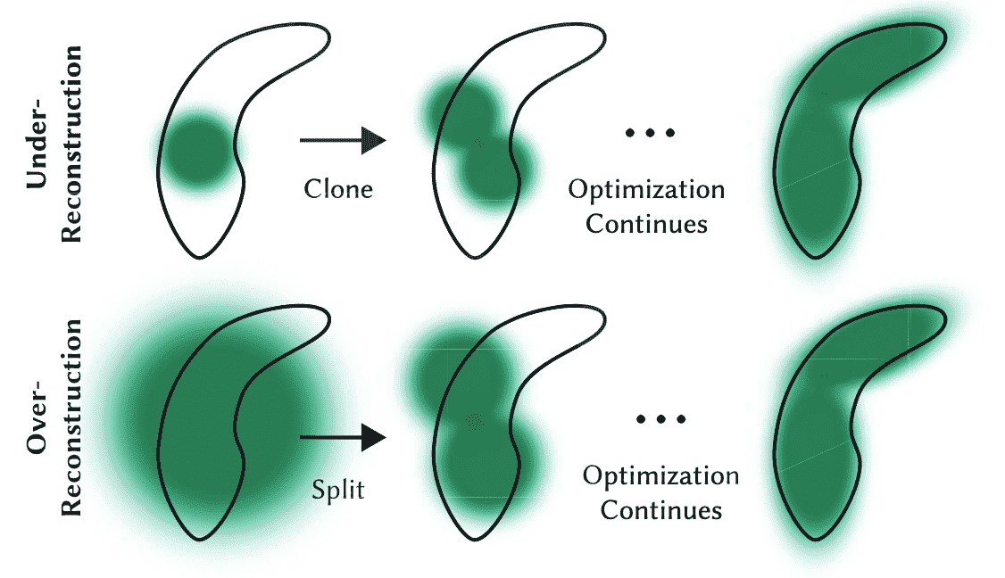
The optimization process relies on iterative cycles of rendering and comparing the resultant image with the training views in the captured dataset. However, due to the inherent ambiguities of 3D to 2D projection, there may be instances where geometry is inaccurately positioned. Therefore, the optimization algorithm must possess the capability to both create geometry and rectify incorrect positioning by either removing or relocating geometry as necessary.

The adaptive density control of Gaussians addresses these challenges by dynamically adjusting the density of splats. In regions with missing geometric features (under-reconstruction), splats are cloned to populate empty areas. Conversely, in regions where Gaussians excessively cover large areas of the scene (over-reconstruction), splats are split to achieve a more refined representation.

$\mathbf{Fig\ 21.}$ Adaptive Gaussian densification scheme (source: )

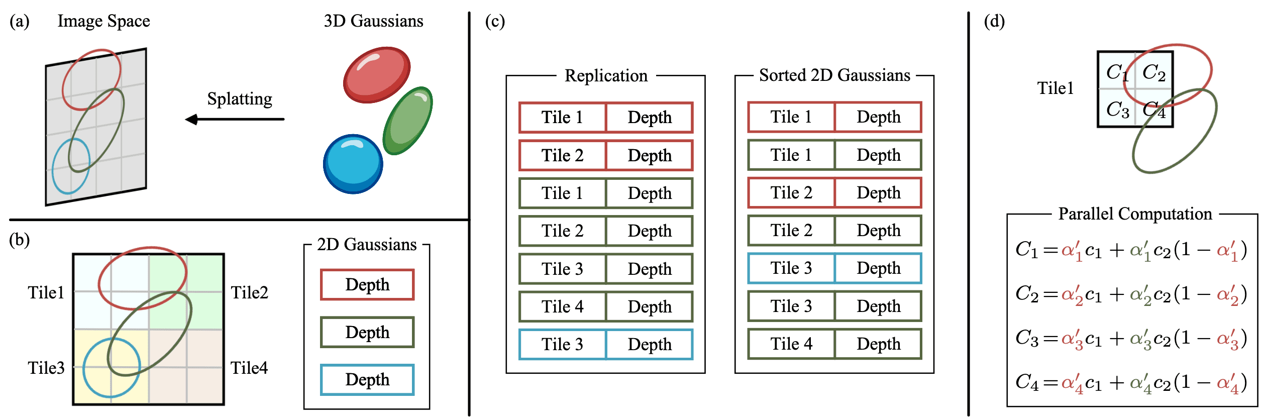
Differentiable Tile-Rasterizer

In 3DGS, the projected Gaussian splats are rendered onto the screen using a differentiable tile-based rasterizer. This process begins by dividing the screen into a disjoint set of $16 \times 16$ tiles. Subsequently, for each tile, the rasterizer culls 3D Gaussians against the view frustum. Gaussians that cover multiple tiles are duplicated, with each copy assigned a corresponding tile ID.

For each pixel in the tile, rays are cast, and the rasterizer proceeds with per-ray depth sorting in parallel. The sorted Gaussians are then rendered in parallel to obtain colored pixels, thereby completing the rendering process.

$\mathbf{Fig\ 22.}$ Differentiable tile-based rasterizer of 3DGS (source: Chen et al. 2024)

By comparing the rendered 2D image and the target image using the following loss function, the 3DGS algorithm automatically propagates training signals throughout the entire forward process:

\[\mathcal{L} = (1 - \lambda) \mathcal{L}_1 + \lambda \mathcal{L}_{\text{D-SSIM}}\]

References

[1] Alexa et al. “Point-Based Computer Graphics SIGGRAPH 2004 Course Notes”
[2] Levoy et al. “The early history of point-based graphics”, Stanford University
[3] Kobbelt and Botsch, “A Survey of Point-Based Techniques in Computer Graphics.”
[4] Zwicker et al. “Surface Splatting”, SIGGRAPH 2001
[5] M. Zwicker, H. Pfister, J. van Baar and M. Gross, “EWA volume splatting,” Proceedings Visualization, 2001. VIS ‘01., San Diego, CA, USA, 2001, pp. 29-538, doi: 10.1109/VISUAL.2001.964490.
[6] Yifan et al. “Differentiable Surface Splatting for Point-based Geometry Processing”, SIGGRAPH Asia 2019
[7] Kerbl et al., “3D Gaussian Splatting for Real-Time Radiance Field Rendering”, SIGGRAPH 2023
[8] Chen et al. “A Survey on 3D Gaussian Splatting”, arXiv 2401.03890
[9] Green et al. “Spherical Harmonic Lighting: The Gritty Details”, Archives of the game developers conference. Vol. 56. 2003.
[10] Ramamoorthi, Ravi. “Modeling illumination variation with spherical harmonics.” Face Processing: Advanced Modeling Methods (2006): 385-424.
[11] Ramamoorthi, Ravi. “Modeling illumination variation with spherical harmonics.” Face Processing: Advanced Modeling Methods (2006): 385-424.