[Graphics] Vast 3D Gaussian

3D Gaussian Splatting works well on small-scale and object-centric scenes, scaling it up to large scenes poses challenges due to limited video memory, long optimization time, and noticeable appearance variations. VastGaussian, proposed by Lin et al. 2024, is the first method for high-quality reconstruction and real-time rendering on large scenes based on 3D Gaussian Splatting.

Problems for large-scale environment

3DGS has several scalability issues when applied to large-scale environments.

1. Limited number of 3D Gaussians
   The rich details of a large scene require numerous 3D Gaussians, but the number of 3D Gaussians is limited by a given video memory.
2. Training times
   3DGS requires sufficient iterations to optimize an entire large scene as a whole, which could be time-consuming, and unstable without good regularizations.
3. Appearance variations of large scenes
   For instance, uneven illumination is commonplace in large scenes, and in such scenarios 3DGS tends to produce large 3D Gaussians with low opacities to compensate for these disparities among different perspectives. Bright blobs often emerge proximate to cameras in images with high exposure, while dark blobs are associated with images of low exposure. These blobs may become unsightly airborne artifacts when observed from novel views.
   
   

   

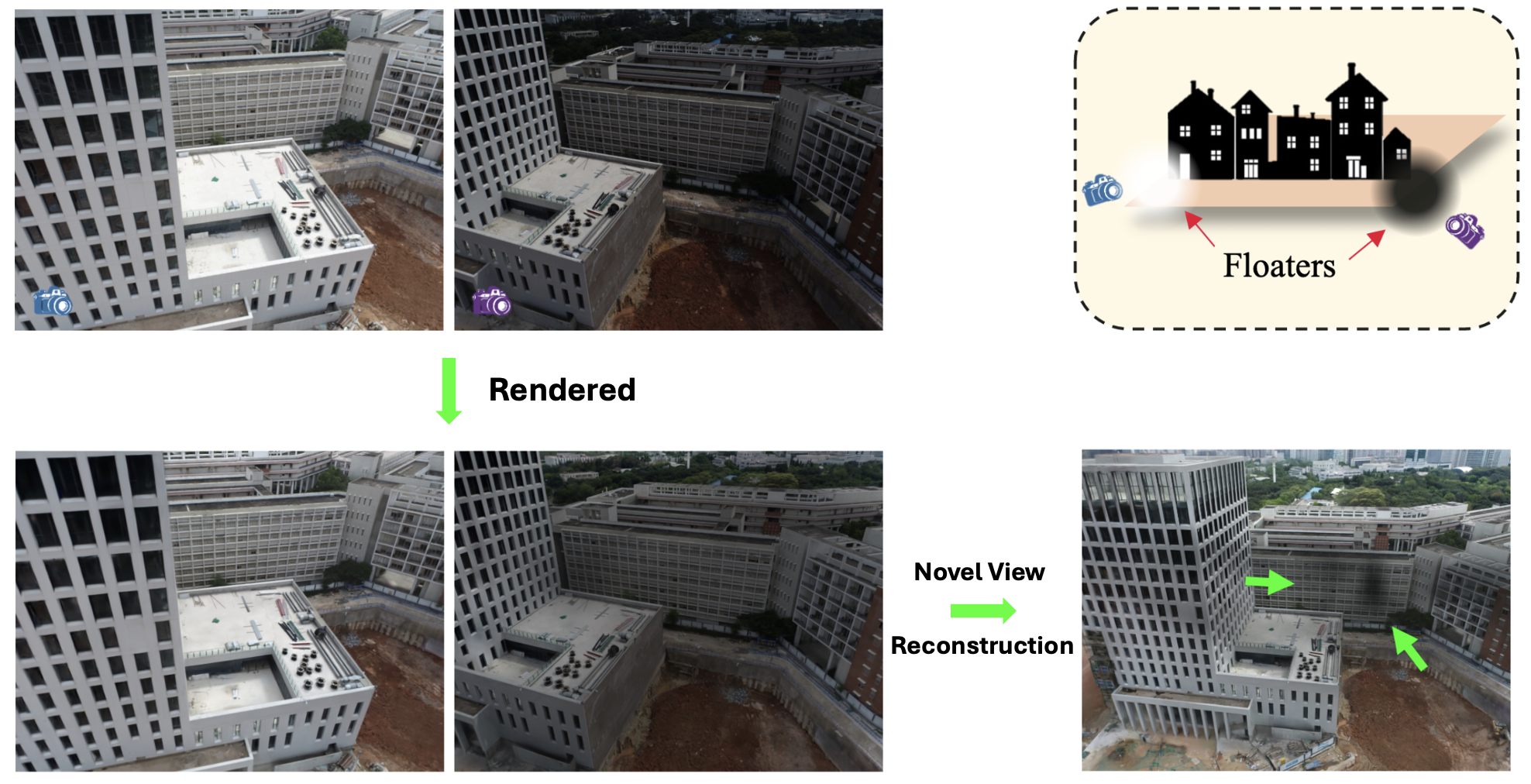
   $\mathbf{Fig\ 1.}$ Appearance variations of large scenes (Lin et al. 2024)
   
   

Vast 3D Gaussians reconstruct a large scene in a divide-and-conquer manner: Partition a large scene into multiple cells, optimize each cell independently, and finally merge them into a full scene.

VastGaussian

Progressive Data Partitioning

VastGaussian partitions a large scene into multiple cells and assign parts of the point cloud $\mathbf{P}$ and views $\mathbf{V}$ to these cells for optimization. Each of these cells contains a smaller number of 3D Gaussians, which is more suitable for optimization with lower memory capacity, and requires less training time when optimized in parallel. This partitioning is termed as progressive data partitioning strategy, and consist of 4 intermediate steps:

$\mathbf{Fig\ 4.}$ Pipeline of progressive data partitioning strategy. (Lin et al. 2024)

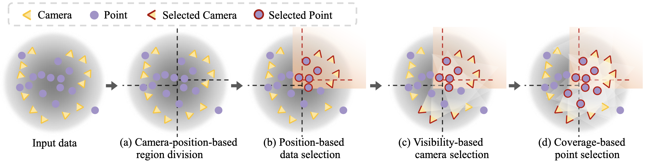
1. Camera-position-based region division
   First, partition the scene based on the projected camera positions on the ground plane, and make each cell contain a similar number of training views to ensure balanced optimization between different cells under the same number of iterations. Specifically, partition the ground plane into $m$ sections along one axis, each containing approximately $\vert \mathbf{V} \vert /m$ views. Then each of these sections is further subdivided into $n$ segments along the other axis, each containing approximately $\vert \mathbf{V} \vert / (m \times n)$ views.
2. Position-based data selection
   Second, assign part of the training views $\mathbf{V}$ and point cloud $\mathbf{P}$ to each cell by expanding its boundaries. Specifically, let the $j$-th region be bounded in a $\ell_j^h \times \ell_j^w$ rectangle; the original boundaries are expanded by a certain percentage, 20% in this paper, resulting in a larger rectangle of size $1.2\ell_j^h \times 1.2\ell_j^w$. We partition the training views $\mathbf{V}$ into $\{ \mathbf{V}_j \}_{j=1}^{m \times n}$ based on the expanded boundaries, and segment the point cloud P into $\{ \mathbf{P}_j \}$ in the same way.
3. Visibility-based camera selection
   For high-fidelity, add more relevant cameras located in other views based on visibility criterion. Given a yet-to-be-selected camera $\mathcal{C}_i$, let $\Omega_{ij}$ be the projected area of the $j$-th cell in the image $\mathcal{I}_i$, and let $\Omega_i$ be the area of $\mathcal{I}_i$; visibility is defined as $\Omega_{ij} / \Omega_{i}$. Those cameras with a visibility value greater than a pre-defined threshold $T_h$ are selected.
   • airspace-agnostic
     A natural and naive solution is based on the 3D points distributed on the object surface; hence airspace-agnostic because it takes only the surface into account. This results in under-supervision for airspace, and cannot suppress floaters in the air.
   • airspace-aware
     Instead, form an axis-aligned bounding box by the point cloud in the $j$-th cell, whose height is chosen as the maximum distance between the highest point and the ground plane. This airspace-aware space takes into account all the visible space, which provides enough supervision for the airspace, thus not producing floaters that are presented in the airspace-agnostic method.
   
   

   

   $\mathbf{Fig\ 2.}$ Two visibility definitions to select more training cameras. (Lin et al. 2024)
   
   The visibility-based camera selection can ensure more common cameras between adjacent cells, effectively eliminating the noticeable boundary artifact of appearance jumping when this method is not employed.
   
   

   

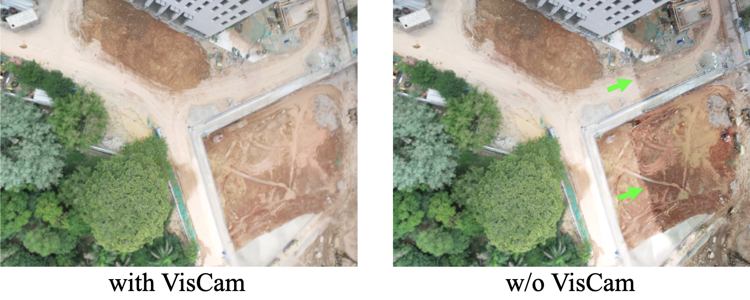
   $\mathbf{Fig\ 3.}$ The visibility-based camera selection can eliminate the appearance jumping on the cell boundaries. (Lin et al. 2024)
   
   
4. Coverage-based point selection
   Then, add the points covered by all the views in $\mathbf{V}_j$ into $\mathbf{P}_j$. Consequently, some objects outside the $j$-th cell can be captured by some views in $\mathbf{V}_j$, and new 3D Gaussians are generated in wrong positions to fit these objects due to depth ambiguity without proper initialization. However, by adding these object points for initialization, new 3D Gaussians in correct positions can be easily created to fit these training views, instead of producing floaters in the $j$-th cell. Note that the 3D Gaussians generated outside the cell are removed after the optimization of the cell.
   
   

   

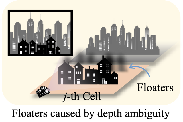
   $\mathbf{Fig\ 4.}$ Floaters caused by depth ambiguity with improper point initialization. (Lin et al. 2024)
   
   

Decoupled Appearance Modeling

To discard appearance variations in the images taken in uneven illumination, NeRF-based methods concatenate an appearance embedding to point-based feature. Inspired by them, the authors proposed decoupled appearance modeling into the optimization process.

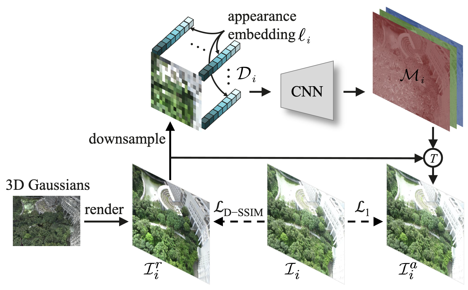
VastGaussian first downsamples the rendered image $\mathcal{I}_i^r$ to not only prevent the transformation map from learning high-frequency details, but also reduce computation burden and memory consumption. Subsequently, it concatenates an appearance embedding $\ell_i$ of length $m$ to every pixel in the 3-channel downsampled image, and obtain a 2D map $\mathcal{D}_i$ with $3 + m$ channels:

\[\mathcal{D}_i = [\mathrm{downsample}(\mathcal{I}_i^r) ; \ell_i] \in \mathbb{R}^{(3 + m) \times h \times w} \text{ where } \ell_i \in \mathbb{R}^{m \times h \times w}, \mathrm{downsample}(\mathcal{I}_i^r) \in \mathbb{R}^{3 \times h \times w}\]

$\mathcal{D}_i$ is progressively upsampled by CNN, generating $\mathcal{M}_i$ that is of the same resolution as $\mathcal{I}_i^r$. Finally, the appearance-variant image $\mathcal{I}_i^a$ is obtained by performing a pixel-wise transformation $T$ on $\mathcal{I}_i^r$ with $\mathcal{M}_i$:

\[\mathcal{I}_i^a = T (\mathcal{I}_i^r; \mathcal{M}_i)\]

For transformation $T$, a simple pixel-wise multiplication was sufficient on the datasets the authors used. The appearance embeddings and CNN are then optimized along with the 3D Gaussians pipeline, independently optimizing all each cells in parallel, using the following loss function:

\[\mathcal{L} = (1 - \lambda) \mathcal{L}_{1} (\mathcal{I}_i^a, \mathcal{I}_i) + \lambda \mathcal{L}_{\text{D-SSIM}} (\mathcal{I}_i^r, \mathcal{I}_i)\]

$\mathbf{Fig\ 5.}$ Decoupled appearance modeling. (Lin et al. 2024)

Seamless Merging

After optimizing all the cells, they are merged into a complete scene. For each optimized cell, the authors eliminate 3D Gaussians spanned outside the original cell region before boundary expansion, as they could become floaters in other cells. Subsequently, we merge the 3D Gaussians from these non-overlapping cells.

$\mathbf{Fig\ 6.}$ Removing 3D Gaussians spanned outside the original cell region.

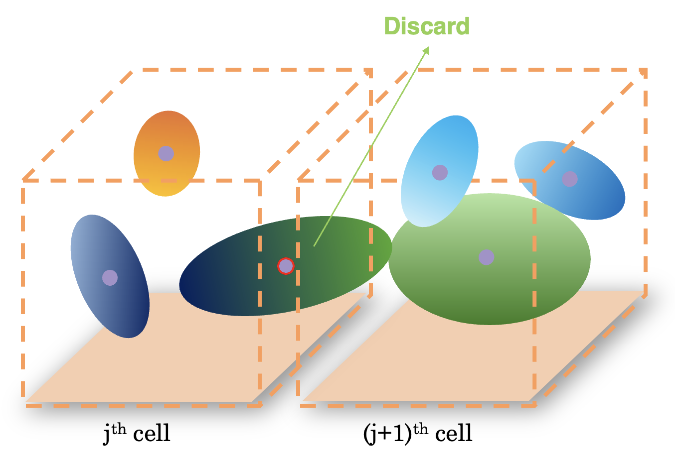
As a result, the merged scene exhibits seamless visual and geometry continuity, without obvious border artifacts, facilitated by the presence of common training views between adjacent cells in data partitioning process. Moreover, the total number of 3D Gaussians within the merged scene can significantly surpass that of the scene trained as a whole, thereby enhancing the reconstruction quality.

Experimental Results

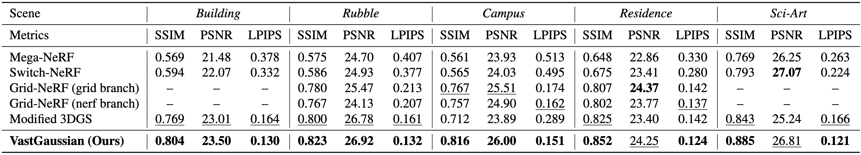
Consequently, VastGaussian surpasses the compared methods across all SSIM and LPIPS metrics by considerable margins, indicating its ability to reconstruct richer details with superior rendering quality. The exceptional quality of VastGaussian can be attributed in part to its extensive number of 3D Gaussians. For example, in the Campus scene, the number of 3D Gaussians in 3DGS is 8.9M, while for VastGaussian, it amounts to 27.4M.

$\mathbf{Fig\ 7.}$ Quantitative evaluation between VastGaussian and previous works. (Lin et al. 2024)

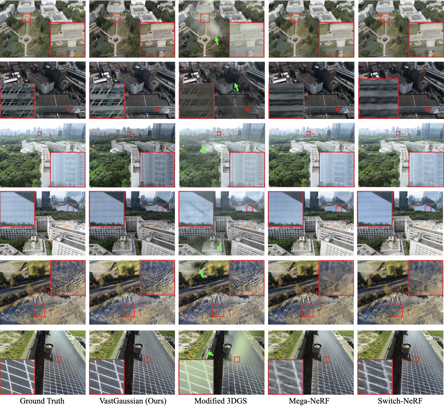
In qualitative comparison, VastGaussian consistently yields clean and visually appealing rendering, whereas NeRF-based methods often lack fine details and produce blurry results, and 3DGS exhibits sharper rendering but generates unsightly artifacts. Albeit VastGaussian exhibits slightly lower PSNR values due to the noticeable over-exposure or under-exposure in some test images, VastGaussian produces significantly better visual quality, sometimes even being clearer than the ground truth, as exemplified by the illustration in the third row of $\mathbf{Fig\ 8}$.

$\mathbf{Fig\ 8.}$ Qualitative comparison between VastGaussian and previous works. ➞ indicates floaters. (Lin et al. 2024)

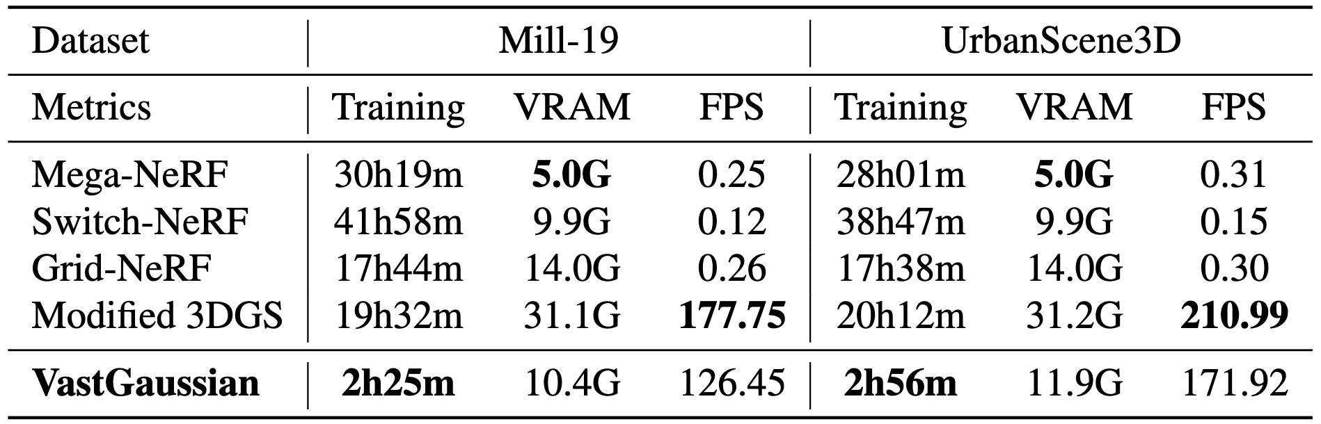
The allure of VastGaussian isn’t just in the stunning scenes, but also in its rendering speed and efficiency. By processing smaller sections of a vast scene concurrently with multiple GPUs, it drastically alleviates computational demands and memory usage. VastGaussian necessitates notably shorter reconstruction times for scenes with photorealistic rendering compared to preceding methods. Futhermore, it achieves real-time rendering with rendering speeds comparable to those of 3DGS, despite containing a greater number of 3D Gaussians in the merged scene.

$\mathbf{Fig\ 9.}$ Comparison of training time, VRAM, and rendering speed. (Lin et al. 2024)

Reference

[1] Lin et al., VastGaussian: Vast 3D Gaussians for Large Scene Reconstruction, CVPR 2024
[2] TheAIGRIDTutorials, Introducing VastGaussian