[CV] Linear Filtering and Detection

In the aftermath of breakthrough in deep learning, the vision model automatically extracts features useful for addressing downstream tasks in images in recent days.

But before emergence of deep learning, especially CNN, engineers hand-programmed the feature or feature extractor traditionally. And in this post, we will delve into one of the most well-known feature extractor called filter.

---

Linear Filtering

The operation of linear filtering actually amounts to convolution neural network, i.e. convolution, or cross-correlation. But distinction is whether the filter is learned itself or not. For example, in deep learning the filter of CNN can be trained from the data by backpropagation. But in traditional approach, filtering, we hand-engineered the appearance of filters.

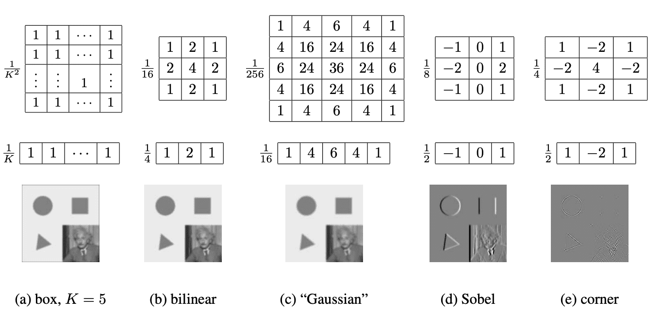
Here are some examples of hand-engineered filters. By adjusting the value, or form of filter, we can set the form of output of filtering as we want:

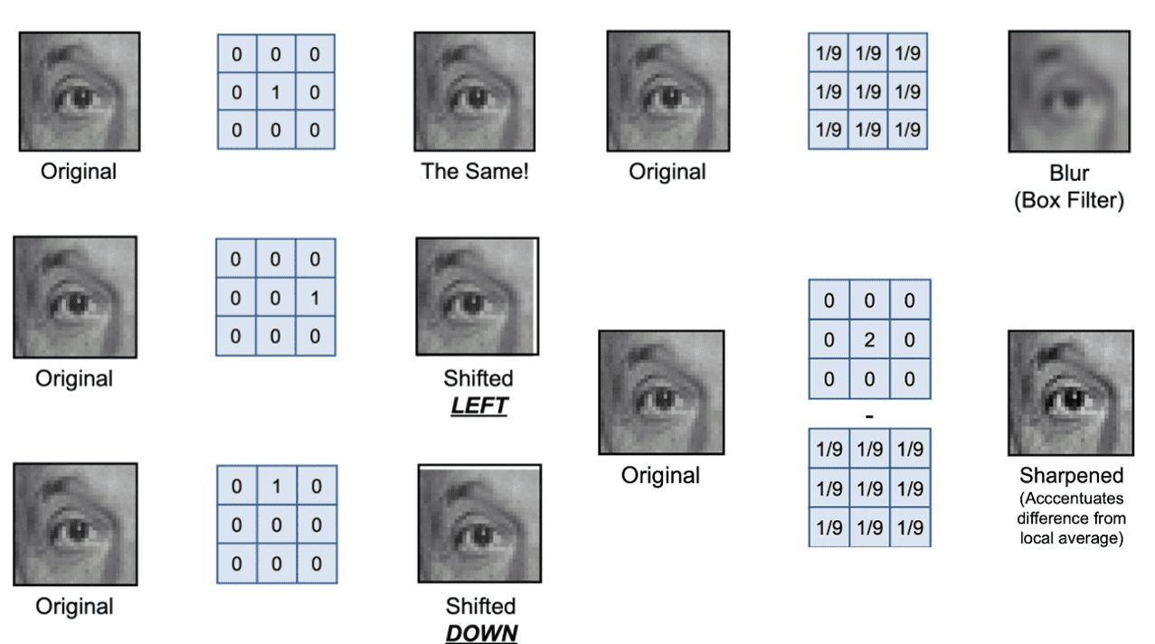
$\mathbf{Fig\ 1.}$ Examples of linear filtering (credit: D. Lowe)

Properties of convolution (linear filtering)

Algebraic property

Convolution (and also cross correlation) has additional nice properties:

• Commutative: $I * F = F * I$
  
• Associative: $(I * F_1) * F_2 = I * (F_1 * F_2)$
  
• Distributive: $I * (F_1 + F_2) = I * F_1 + I * F_2$
  
• Scalars factor out: $k I * F = I * kF = k (I * F)$
  

Here, $I$ is an image and $F, F_1, F_2$ are filters. And these properties yield some instrumental implications in linear filtering.

Linearity

By distributive property $I * (F_1 + F_2) = I * F_1 + I * F_2$, it is the fact that linear filtering is a linear operator:

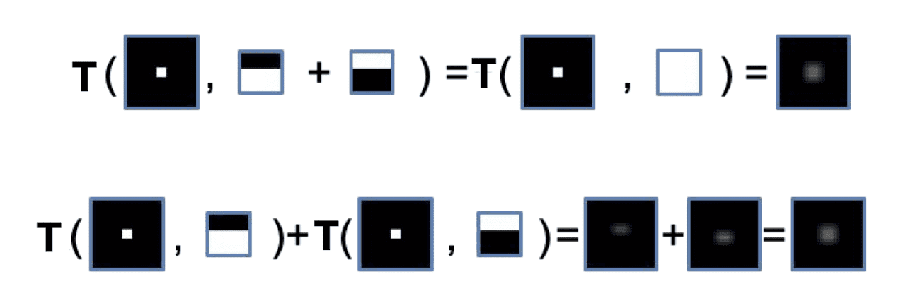
$\mathbf{Fig\ 2.}$ Linearity of linear filtering

Hence, it implies that both cross correlation and convolution operators can always be represented as a matrix-vector multiplication.

Shift invariance

Since shift operator can be written as applying filter, we can obtain shift invariance property of linear filtering, i.e. $\text{shift}(I * F) = \text{shift}(I) * F$ from associativity $(I * F_1) * F_2 = I * (F_1 * F_2)$ of convolution:

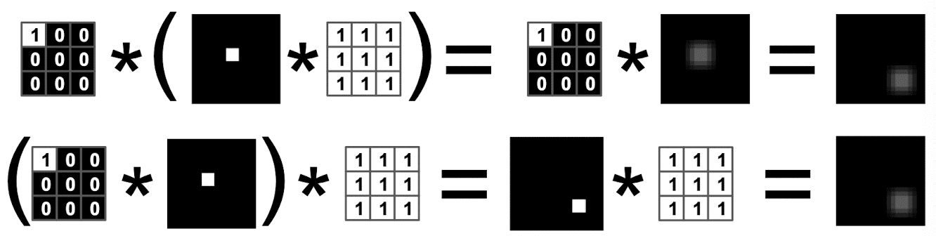
$\mathbf{Fig\ 3.}$ Shift invariance of linear filtering

Seperability

As the filter slides over the entire image, a convolution operator requires $K^2$ (multiply and add) operations per pixels where $K$ is the size of filter.

However, one interesting property in linear filters is that some linear filters are separable. If the filter is separable, it can be separated into more than two matrices, similar with matrix decomposition.

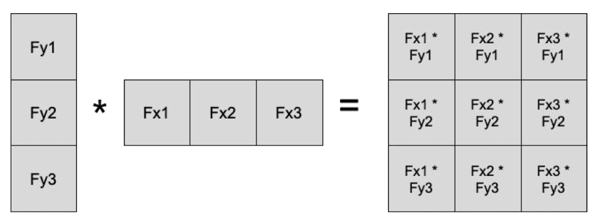
$\mathbf{Fig\ 4.}$ Separablity (credit: D. Fouhey)

So, applying a separable filter to image is equivalent to applying the separated filters sequentially. For example, if a filter is decomposed into outer products of 1D vectors, it will be much efficient that applying 2D filter to image. ($3 \times 3$ \to $3 + 3$ multiplications per pixel)

The figure outlined below shows some examples for separable filters. 2D Gaussian filter is one of examples of separable linear filter:

\[\begin{gathered} \text { Filter }_{i j} \propto \frac{1}{2 \pi \sigma^2} \exp \left(-\frac{x^2+y^2}{2 \sigma^2}\right) \\ \longrightarrow \\ \text { Filter }_{i j} \propto \frac{1}{\sqrt{2 \pi} \sigma} \exp \left(-\frac{x^2}{2 \sigma^2}\right) \frac{1}{\sqrt{2 \pi} \sigma} \exp \left(-\frac{y^2}{2 \sigma^2}\right) \end{gathered}\]

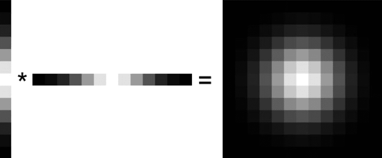
$\mathbf{Fig\ 5.}$ Separability of 2D Gaussian

$\mathbf{Fig\ 6.}$ Separable linear filters

Image processing with filters

From now on, we will utilize these filters to image.

Remove noises

Let’s remove noises which is called salt and pepper noises in the image.

$\mathbf{Fig\ 7.}$ Image with salt and pepper noise (credit: D. Fouhey)

Then, how can we design a filter that reduces the noise? If the noises are randomly distributed, we can take the local average by box filter.

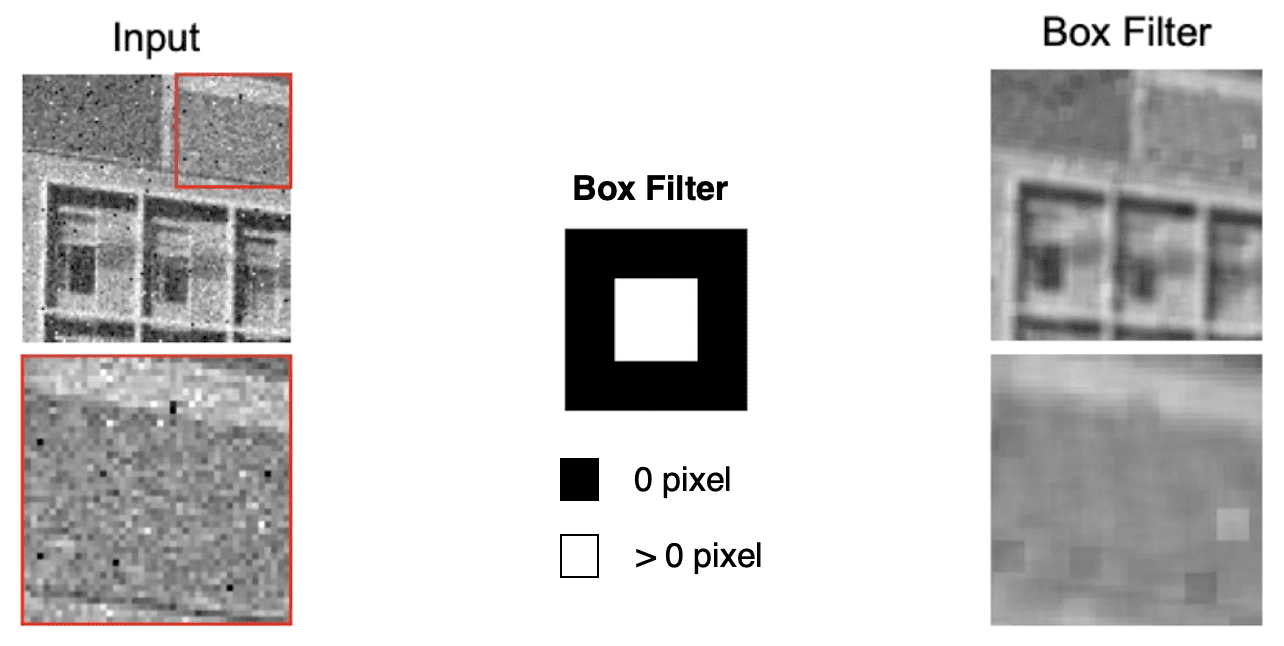
$\mathbf{Fig\ 8.}$ Removing noises by local averaging with box filter

But local averaging may remove details too much, and we can observe some blocky artifacts. Instead of rectangle box filter, we may use Gaussian filter which has much smoother boundary. Due to form of gaussian function, it amounts to take the local weighted average to the image. We can see that the blurred image of Gaussian filter is much smoother than that of box filter.

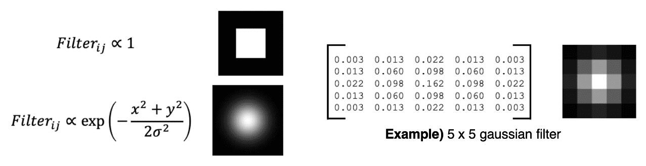
$\mathbf{Fig\ 9.}$ Gaussian filter

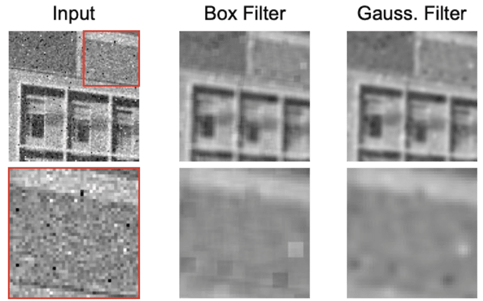
$\mathbf{Fig\ 10.}$ Comparison with box filter

Note that the standard deviation $\sigma$ of Gaussian filter acts as a hyperparamter. Indeed, it defines how much we want to blur the image, i.e. degree of blurness.

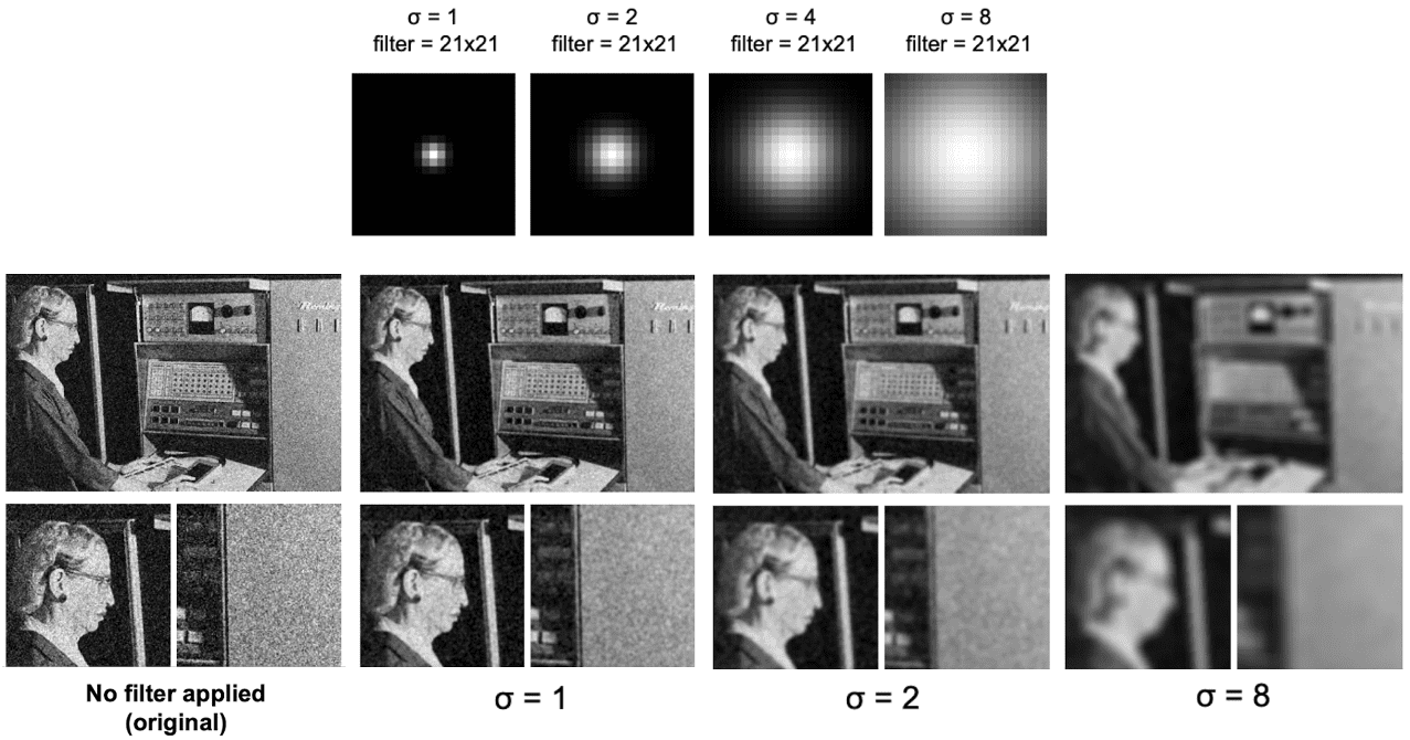
$\mathbf{Fig\ 11.}$ Effect of standard deviation in Gaussian filter (credit: D. Fouhey)

Detection with filters

Linear filters can be also utillized in order to decting interesting point of image. In this post, we will focus on corners.

Edge

Edge is a set of points lies in the boundary of two distinctive regions. Although it is not an interesting point, but we will first design a filter that detects edges for further development to detect much complicated structures. Then the first thing we need to consider is: how do we define the edges? What makes an edge?

One instrumental thing, which may be a definition of edge, is that pixel entensity will change dramatically in $x$ or $y$ direction on the edge.

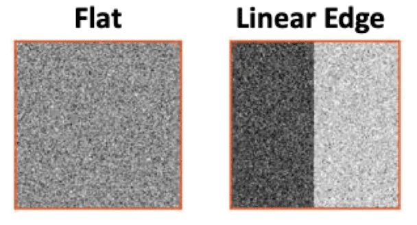
$\mathbf{Fig\ 12.}$ Linear Edge

Hence, to detect an edge, it is reasonable to measure variability of pixel values in $x$ or $y$ direction.

Image Gradient

We define image gradient that quantifies the direction and magnitude of intensity changes. For the pixel intensity at $(x, y)$ pixel, image gradient is defined as:

\[\begin{aligned} \nabla I(x, y)=\left[\begin{array}{l} \frac{\partial I(x, y)}{\partial x} \\ \frac{\partial I(x, y)}{\partial y} \end{array}\right] \end{aligned}\]

where $I(x, y)$ denotes the pixel intensity at $(x , y)$ pixel. Thus image gradient indicates how much the intensity of the image changes as we go horizontally at $(x,y)$. Note that the size of this partial derivatives matrix is equal to the size of input image.

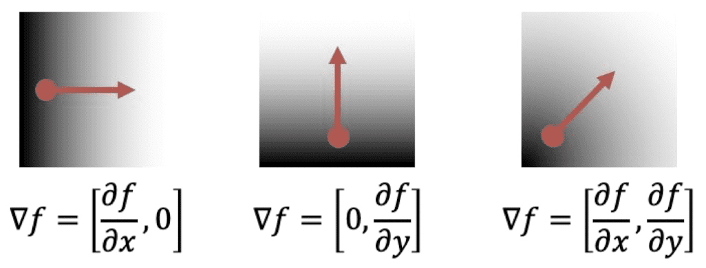
$\mathbf{Fig\ 13.}$ Visualization of image gradient

Then we can basically calculate image gradient (partial derivative) using filters. Recall that the definition of partial derivative is

\[\begin{aligned} \frac{\partial I(x, y)}{\partial x} = \lim_{\varepsilon \to 0} \frac{I(x + \varepsilon, y) - I(x,y)}{\varepsilon} \end{aligned}\]

Since, pixel coordinates are discretized, i.e. $1$ is the smallest unit for the pixel, this partial derivative can be approximated by

\[\begin{aligned} \frac{\partial I(x, y)}{\partial x} \approx \frac{I(x + 1, y) - I(x,y)}{1} \end{aligned}\]

And it is also equivalent to

\[\begin{aligned} \frac{\partial I(x, y)}{\partial x} \approx \frac{I(x + 1, y) - I(x - 1,y)}{2} \end{aligned}\]

In terms of filter, the above operations can be implemented by filters:

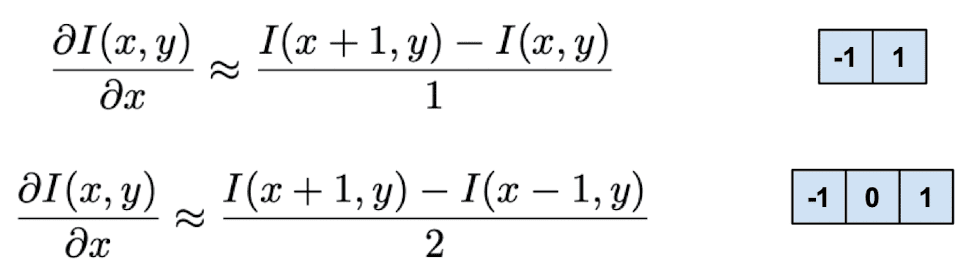
$\mathbf{Fig\ 14.}$ Computing image gradient with filters

Extending to 2D, the following filters approximate the image gradient of input image:

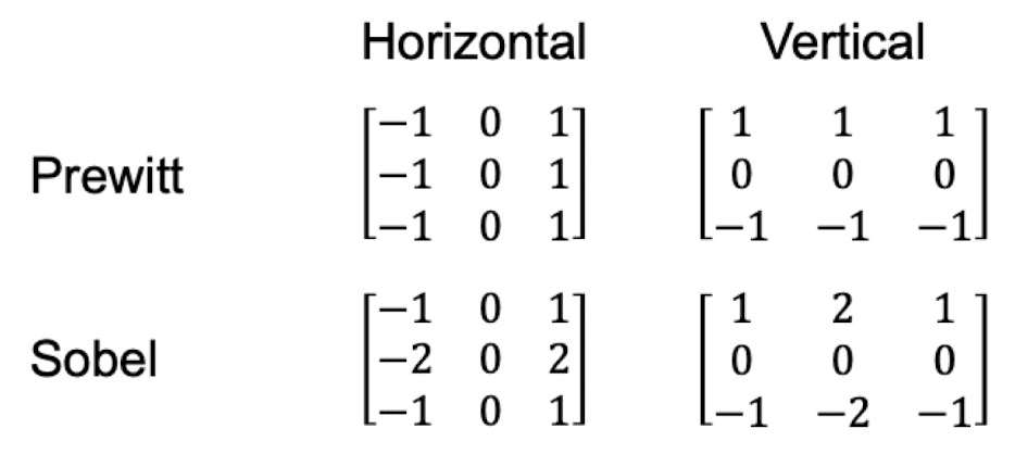
$\mathbf{Fig\ 15.}$ 2D image gradient filters

Then we can detect vertical and horizontal edges from the image by applying image of gradient filters individually. Here are results of image of gradient:

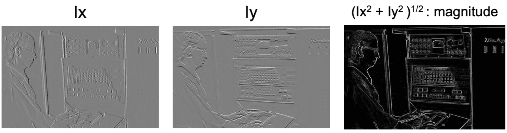
$\mathbf{Fig\ 16.}$ Result of image gradient

Derivatives of Gaussian (DoG)

However, the main issue of image gradient is, it is too sensitive to noises. Consider the following 1d signal, for example:

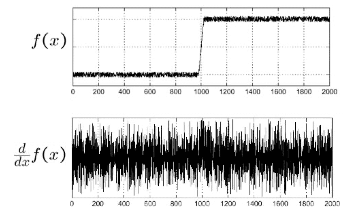
$\mathbf{Fig\ 17.}$ 1D noise $f(x)$ and its gradient $\frac{d}{dx} f(x)$

It looks like clear step signal, but if we take a partial derivative to this we get noisy output in contrast to what we expect. A simple way to solve this is to apply smoothing (blurring) such as Gaussian filter to reduce the impact of the noise.

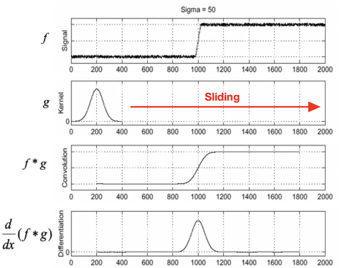
$\mathbf{Fig\ 18.}$ Applying Gaussian filter and computing image gradient

where $g$ is Gaussian filter. By associativity of linear filter and since applying partial derivative can be represented as applying a filter, we can make it one pass:

\[\begin{aligned} \frac{d}{dx} (f * g) = f * \frac{d}{dx} g \end{aligned}\]

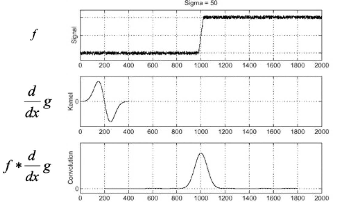
$\mathbf{Fig\ 19.}$ One pass of Gaussian filter and image gradient

For 2D case,

\[\begin{aligned} I_x = \frac{\partial}{\partial x} (G * I) &= D_x * (G * I) = (D_x * G) * I = (\frac{\partial}{\partial x} G) * I \\ I_y = \frac{\partial}{\partial y} (G * I) &= D_y * (G * I) = (D_y * G) * I = (\frac{\partial}{\partial y} G) * I \\ \end{aligned}\]

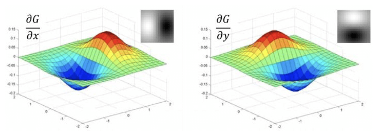
$\mathbf{Fig\ 20.}$ Example of Derivative of Gaussian Filter with respect to x and y direction (credit: [2])

where $I$ is an image, $G$ is a Gaussian filter, and $D_x$ and $D_y$ are filters correspond to image of gradient of $x$ and $y$ axis, respectively. The following figure is the result of applying derivatives of Gaussian.

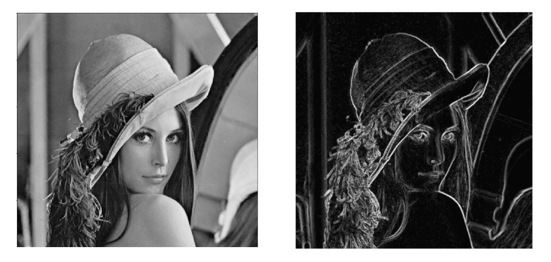
$\mathbf{Fig\ 21.}$ result of applying gradient of Gaussian (credit: [2])

Corner (Harris Corner Detection)

Let’s extend it further to corner detection. The corner is basically the junction of contours (edges). And the contours can have junctions only if they have a different orientation, i.e. the points whose local neighborhood exhibit distinct edged directions. Thus it can be the one of the good local features to match due to uniqueness or distinctiveness in its pattern compared to other plane area or the areas with only edges. And by discovering these corners, then we can describe the image using the unique set of local features and by matching these local features, we can identify that this is the same image.

So, to be able to detect the corner, we first need to characterize the corner. One possible way is that starting from the original location, we move the filter by a few pixels around a local neighborhood and measure the difference within the filter area as follows:

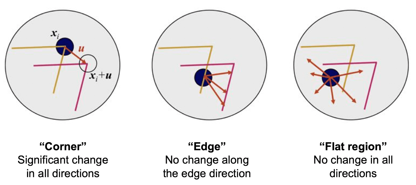
$\mathbf{Fig\ 22.}$ Characterizing corner

To measure the change of intensity for the shift $u$ and $v$, we define the small window $w(x, y)$ instead of the entire image and measure the differences within this small window corresponding to blue dot in the figure above. It is because we are not moving the entire image, but we are moving the filter that is a candidate for the corner and then measure the difference within it. And then we are taking the average of this intensity value differences over the window size. As a mathematical formula,

\[\begin{aligned} E(u, v) = \sum_{x, y} w(x, y) \cdot \left(I (x + u, y + v) - I(x, y) \right)^2 \end{aligned}\]

where $(x, y)$ denotes pixel locations within the window. The intensity difference $(I (x + u, y + v) - I(x, y))^2$ will measure the change of pixels. For nearly constant patches, it will be near $0$, and for very distinctive patches, it will be large.

And there are few choices for window $w$: for example, if window function is uniform ($1$ in window, $0$ outside), $E(u, v)$ is just an average of change of intensity over pixels. But in some cases, we may want to measure the differences over the center location of the filter more heavily than the others. Then we can define our window function with Gaussian. It is more robust against the noises because it prioritizes the difference near the center.

$\mathbf{Fig\ 23.}$ Choice of window functions

For the next step, we are going to apply tailor first-order expansion to calculate this more efficiently:

\[\begin{aligned} E(u, v) & =\sum_{x, y} w(x, y)(I(x+u, y+v)-I(x, y))^2 \\ & \approx \sum_{x, y} w(x, y)\left(I(x, y)+u I_x(x, y)+v I_y(x, y)-I(x, y)\right)^2 \\ & =\sum_{x, y} w(x, y)\left(u^2 I_x^2(x, y)+2 u v I_x(x, y) I_y(x, y)+v^2 I_y^2(x, y)\right) \\ & =\sum_{x, y} w(x, y)\left[\begin{array}{c} u \\ v \end{array}\right]^{\mathrm{T}}\left[\begin{array}{cc} I_x^2(x, y) & I_x(x, y) I_y(x, y) \\ I_x(x, y) I_y(x, y) & I_y^2(x, y) \end{array}\right]\left[\begin{array}{l} u \\ v \end{array}\right] \\ & =\left[\begin{array}{c} u \\ v \end{array}\right]^{\mathrm{T}}\left(\sum_{x, y} w(x, y)\left[\begin{array}{cc} I_x^2(x, y) & I_x(x, y) I_y(x, y) \\ I_x(x, y) I_y(x, y) & I_y^2(x, y) \end{array}\right]\right)\left[\begin{array}{l} u \\ v \end{array}\right] \end{aligned}\]

If we look closely the last term and inside of $[u \; v]$, we get

\[\begin{aligned} M = \sum_{x, y} w(x, y)\left[\begin{array}{cc} I_x^2(x, y) & I_x(x, y) I_y(x, y) \\ I_x(x, y) I_y(x, y) & I_y^2(x, y) \end{array}\right] \end{aligned}\]

which is the outer product of image gradient with respect to $x$ and $y$ coordinates:

\[\begin{aligned} M = \sum_{x, y} w(x, y) \cdot \left[\begin{array}{c} I_x(x, y) \\ I_y(x, y) \end{array}\right] \times \left[\begin{array}{c} I_x(x, y) \\ I_y(x, y) \end{array}\right] \end{aligned}\]

So, by looking at this inside term $M$, we can see whether it contains the edge or flat area or the corner. For example, this is the distribution of the image gradient components:

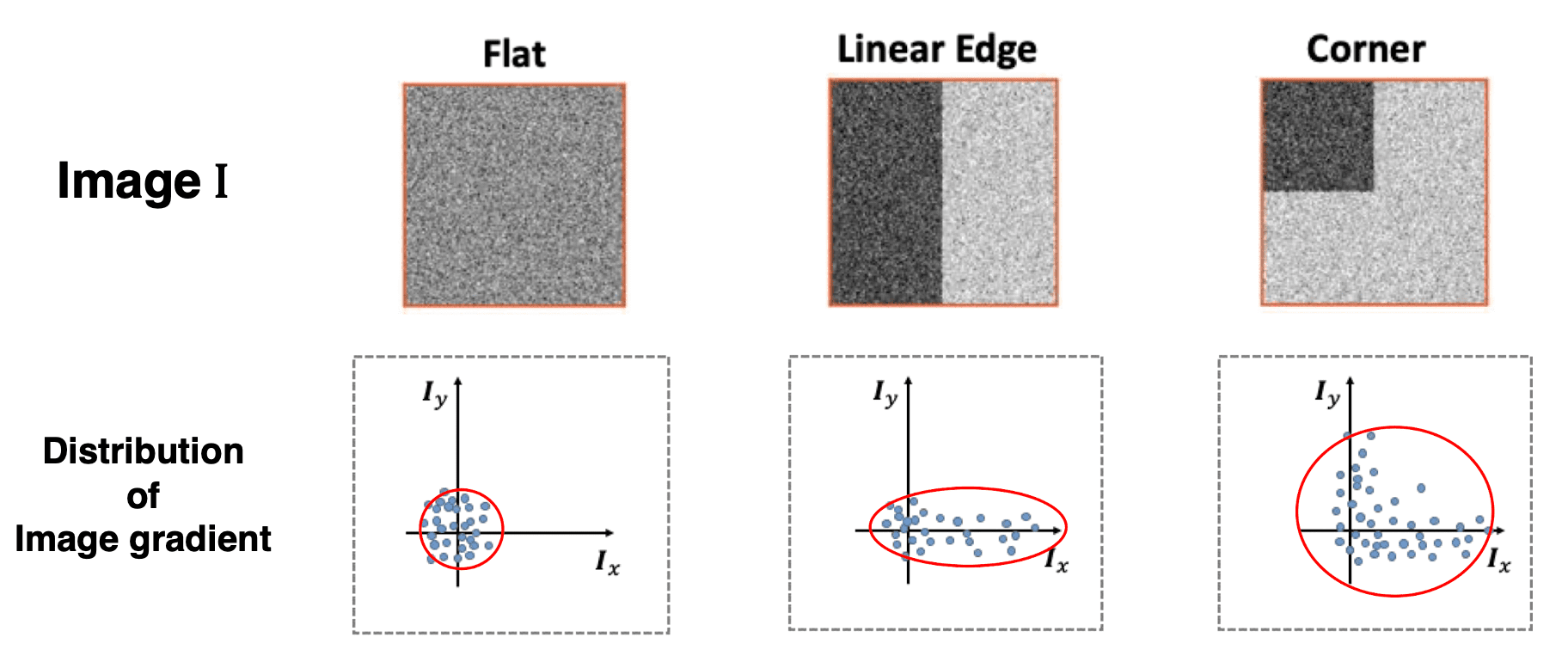
$\mathbf{Fig\ 24.}$ Distribution of components of image gradient

So as to analyze it, we decompose matrix $M$ into the collection of eigenvectors and corresponding eigenvalues, which basically characterize the distribution of derivatives. Note that there always exists an eigenvalue decomposition of $M$ as $M$ is the weighted sum of symmetric matrices.

\[\begin{aligned} M=\sum_{x, y} w(x, y)\left[\begin{array}{cc} I_x^2 & I_x I_y \\ I_x I_y & I_y^2 \end{array}\right]=V\left[\begin{array}{cc} \lambda_1 & 0 \\ 0 & \lambda_2 \end{array}\right] V^{\mathrm{T}} \end{aligned}\]

Then the two eigenvalues determine the shape and the size of the principle component ellipse. It is outlined below:

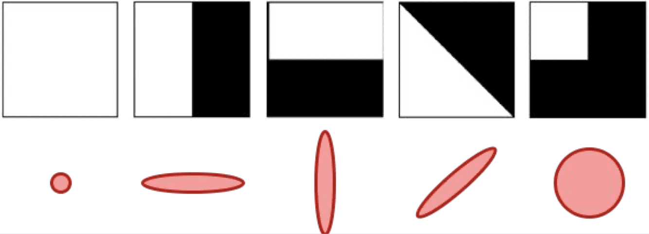
$\mathbf{Fig\ 25.}$ Principle component ellipse and edges and corners

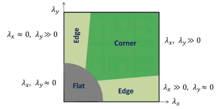
For instance, if it has some high responses over a certain direction and small responses over the other direction then basically you get a high eigenvalue for one direction and small eigenvalue for the other eigenvector.

Hence now we know that the difference between two eigenvalues are important to detect the corner. These differences in terms of the eigenvalues can be measured by a heuristic way:

\[\begin{aligned} R = \text{det}(M) - k \cdot \text{tr}(M) = \lambda_1 \lambda_2 - k \cdot (\lambda_1 + \lambda_2)^2 \end{aligned}\]

$\mathbf{Fig\ 26.}$ Corner response

In summary, the following figure shows the overall pipeline for corner detection, which is referred to as Harris corner detection.

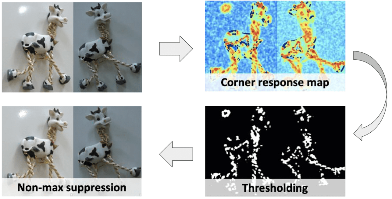
$\mathbf{Fig\ 27.}$ Harris Corner Detection

Reference

[1] CS 376: Computer Vision of Prof. Kristen Grauman
[2] jun94, [CV] 3. Gradient and Laplacian Filter, Difference of Gaussians (DOG)
[3] [계산사진학] Image Filtering - Image Gradients and Edge Detection
[4] Szeliski, Richard. Computer vision: algorithms and applications. Springer Nature, 2022.