[CV] Blob detection and SIFT

In this post, we are going to dive into the different ways for detecting corner and how we can describe the characteristics of the local neighborhood around the corners, which representation is called SIFT, one of the most popular representations before the deep learning era.

Blob

Blob is the image region that is either brighter or darker than the surrounding, which gives us some unambiguity in terms of image matching. More roughly, blobs are regions that are distinguishable from surroundings.

$\mathbf{Fig\ 1.}$ Example of blob detection

To design the filter for detecting blobs, let’s recall the filter of edge detection. Consider 1D signal for input image. In case of the edge, we have some discontinuity at middle jump point. And we discussed earlier that the derivative of the gaussian can be one solution for that case.

$\mathbf{Fig\ 2.}$ Recall: edge detection

Similarly, for the darker blobs, how can we design the detector?

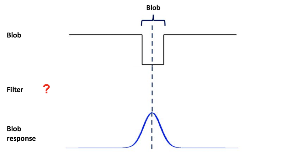
$\mathbf{Fig\ 3.}$ Darker blob detection

Let’s try the gaussian filter first, but slightly modified version.

If we add the filters of the second order derivative as follows:

and we call it laplacian of the gaussian

In case of the 2d isotropic standard gaussian,

~ 식

Laplacian of 2D isotropic standard Gaussian distribution is

~ 식

Now, let’s apply Laplacian of gaussian for the blob. If you apply the laplation of the gaussian it’ll be near zero. Then once it hits the blob once, it outputs the high responses for the region.

사진

But the problem is that depending on how you set the variance the scale of the Laplacian of the gaussian, you may get different types of outputs. If the scale of the Laplacian of Gaussian is too small, then the output value will be almost same as the flat area.

사진

So we have to find the right scale for detecting the blops in different sizes. Within the same image, we get different plops with different sizes and we cannot discover all of them using the single Laplacian of the Gaussian. To select the optimal scale, we may actually use the property that the output value of the filtering is maximized when it matches the right scale to analytically compute the proper scale of the filter given the size of the block.

Let’s think about some blobs in circle for simplicity and denote the radius of the blob by $r$.

Then the response of the laplacian filter with respect to different scale is computed:

The problem, however, is that if you increase the scale of the Laplacian filter then you would get smaller responses due to We saw it laplacian of 2d isotropic 머시기.

So, we normalize it to compensate for it through multiplying variance over the Laplacian of the Gaussian. It will maintain the maximum value of the Laplacian Gaussian filter.

Finally, the following figure shows the result of single scale blob detection. We can see that it has strong responses around the blob with the proper size but there are weak responses for some tiny blops or large blops.

Identifying the right scale

To be able to detect the blops in multiple scales what we can do is that we can apply this Laplacian of gaussian filter with multiple scales and get 2D response map at multiple scales of the filters.

사진

Then it shows how the response value changes into 2D neighborhood and as well as the scale direction scale axis. If it is the maximum value around both the spatial neighborhood and the scale dimension then we can say that the blop is correctly detected and the size of the blop is matched to that scale. The following figure shows the result after we apply this.

Examples of blob

SIFT

Once we have detected the interest points, we want to utilize it, in other words, describe or summarize our image using these local interest points. So, how do we describe the patterns around the local features?

Consider that we have an input image and we obtained some bloops as a result of the blop detection. We may want to describe the local textures around the blops.

When we design the descriptor of the local interest point we want consistent representation of objects invariant to scale variation, illumination, rotation, etc. To do that, we are going to discuss about SIFT, Scale invariant feature transform.

사진

The idea of this sift feature is very simple and again, it’s heuristic. The high level idea is that from the input image patch, we measure the distribution of the edge orientations within the local window.

(1) Finding a scale-space extrema (blob detection)

Instead of Laplacian of Gaussian, Difference of Gaussian (DoG): the difference between two Gaussians with different variances is used in SIFT.

식

If you measure the difference between gaussian with different scale it’s roughly proportional to the laplacian of the gaussian. So, instead of calculating the laplacian of the gaussian, we can approximate this is laplation of the gaussian with the two gaussians efficiently.

(2) Keypoint filtering

once you get the responses from this difference of the gaussians you can basically threshold the key points

(3) Orientation assignment

Once you get the blobs, you can describe the characteristics of the patch inside of the blob using the orientation of the gradients. So, by measuring their magnitude, we get the magnitude of the edge responses and can get the orientation of the edges from that.

식

And then, we want to first measure which orientation of the edge is most dominant orientation. To do that, we build a histrogram of orientations and pick the highest peak as follows:

사진

Most common hyper (Build a histogram 말하는거)

This is some detailed, most common hyperparameter of this sift picture. We usually divide the local patchs around the blob using the four by four quadrant. And when you build a histogram for each quadrant we use 8 bins for the orientations and normalize the number of components in the histogram to sum to one.

Sometimes the dimension of the entire concatenated histogram could be very large in which case we apply some optional dimensional reduction like PCA.