[CV] Motion and Optical Flow

In this post and next few posts, we will discuss about some problems in the video domain such as visual object tracking or action recognition. And as a start we delve into the way how to compute the motion in a video and algorithms to compute per-pixel motion.

Motion and Optical Flow

So far we usually denote our image into the 3D tensor: rgb channel, width and height. In case of video, it is basically the collection of the frames and each of the frame is an image, so we represent the video in terms of 4D tensor.

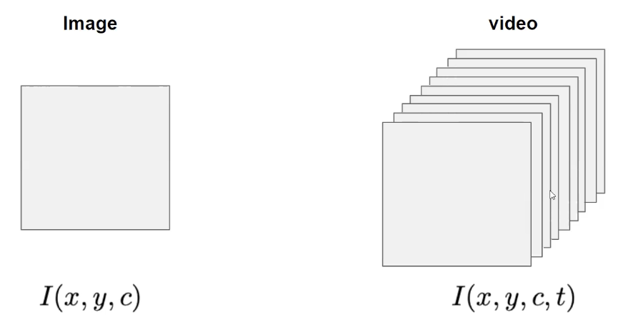
$\mathbf{Fig\ 1.}$ Video Representation

Hence, additional one dimension will be extended which corresponds to the time. And now we have patterns not only in the spatial domain, but also temporal domain.

And some patterns we are interested in the temporal domain are usually about the motion. A motion is a phenomenon that an object changes its position over time. And in this post we will focus on the optical flow which calculates the pixel-wise motion (displacement) and is the most general and challenging version of motion estimation:

$\mathbf{Fig\ 2.}$ Optical Flow of Traffic (source: Chuan-en Lin)

Optical Flow equation

Then how can we quantify a pixelwise displacement? Let’s denote pixel at $x$ and $y$ coordinate as $(x, y)$. And assume the pixel at $(x, y)$ in time $t$ is moving, and it shifts to new location $(x + dx, y + dy)$ at time $t + dt$:

$\mathbf{Fig\ 3.}$ Our optical flow problem (source: Chuan-en Lin)

Here, $I(x, y, t)$ denotes the intensity of pixel at $(x, y)$ for time $t$. To make this high-level problem more simpler, we will suppose two key assumptions:

1. Color/brightness constancy: point at time $t$ looks same at time $t + 1$
2. Small motion: points do not move very far between temporally adjacent frames

Then, by exploiting brightness constancy assumption,

\[\begin{aligned} I(x, y, t) = I(x + dx, y + dx, t + dt) \end{aligned}\]

And by approximating the RHS by first-order taylor expansion,

\[\begin{aligned} I(x, y, t) &= I(x + dx, y + dx, t + dt) \\ &\approx I(x, y, t) + \frac{\partial I}{\partial x} dx + \frac{\partial I}{\partial y} dy + \frac{\partial I}{\partial t} dt \end{aligned}\]

Obviously, this is the approximation so the accuracy of this equality depends on the magnitude of differentials $dx$, $dy$ and $dt$. ($dx$ and $dy$ should not be too long, which concides with our second assumption) By rewriting it and defining a motion vector $(u, v) = \left( \frac{dx}{dt}, \frac{dy}{dt} \right)$, we obtain an equation called optical flow equation:

\[\begin{aligned} 0 \approx I_x u + I_y v + I_t \text{ where } (u, v) = \left( \frac{dx}{dt}, \frac{dy}{dt} \right) \end{aligned}\]

or equivalently,

\[\begin{aligned} \nabla I \; \left[\begin{array}{l} u \\ v \end{array}\right] = \left[\begin{array}{ll} I_x(\mathbf{p}) & I_y(\mathbf{p}) \end{array}\right]\left[\begin{array}{l} u \\ v \end{array}\right]=-I_t(\mathbf{p}) \end{aligned}\]

Apeture problem

Here, we know that $I_x$ and $I_y$ are horizontal and vertical image gradient, respectively and calculation of image gradient can be done by using only linear filtering efficiently.

Similarly, $I_t$ can be approximated similarly with image gradient by $I_t \approx I(x, y, t + 1) - I (x, y, t)$. Therefore we can solve this optical flow equation. But the remaining problem is that there are infinitely many solutions for this equation (one equation, but two unknown variables $u$ and $v$).

And such a undecidability implies well-known problem in optical flow that is referred to as apeture problem. Let’s visualize $\nabla I$ as a 2D vector, and envision a line orthogonal to $\nabla I$.

Then for any $[u^\prime, v^\prime]$ on the line, the inner product $(\nabla I)^\top [u^\prime, v^\prime] = 0$. In this formulation, for any motion $[u, v]$, there is always ambiguity since

\[\begin{aligned} (\nabla I)^\top [u, v] = (\nabla I)^\top [u + u^\prime, v + v^\prime] \end{aligned}\]

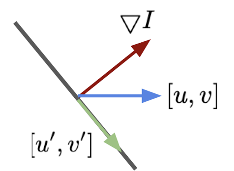
$\mathbf{Fig\ 4.}$ Visualization of vectors

More intuitive figures are given below. Let’s focus on the sky-blue object behind the green aperture. It is straightforward that the sky-blue object is clearly shifted to the left.

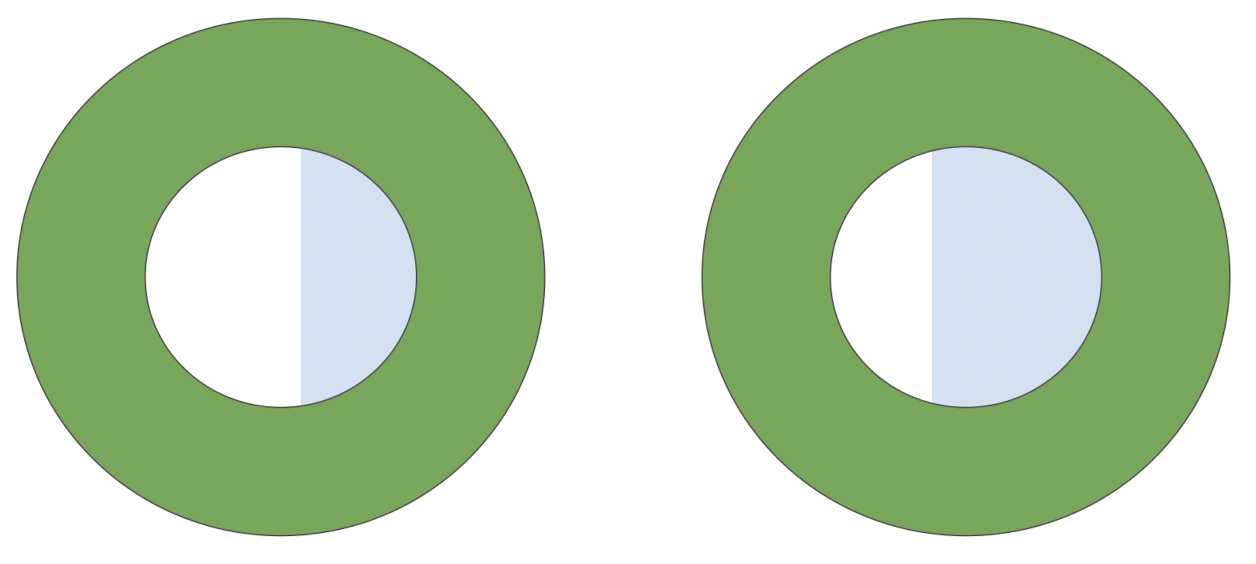
$\mathbf{Fig\ 5.}$ Aperture problem

But, if the green aperture is removed, there are infinitely many possibilities such as horizontal move and digonal moves due to blind spot created by green object:

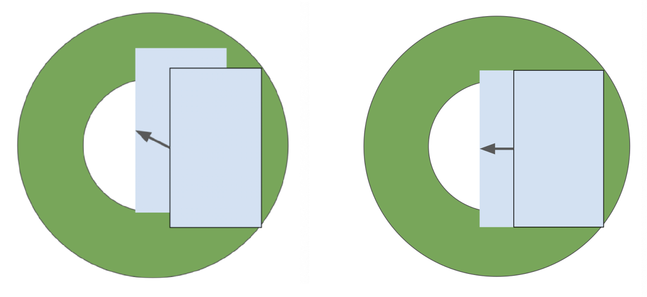
$\mathbf{Fig\ 6.}$ Aperture problem

Lucas-Kanade Algorithm

The image brightness constancy assumption only provides the optical flow component in the direction of the spatial image gradient. Therefore, to solve the optical flow equation we need more directions of gradients to get more equations, rather than the image gradient only.

So as to introduce additional condition, assume spatial coherence: pixels in a small local neighborhood have the same motion, i.e. $[u \; v]$. Then we can use local window for additional equations, for instance, for $5 \times 5$ local pixel neighborhood of 25 pixels $p_1, \dots, p_{25}$:

\[\begin{aligned} \underbrace{\left[\begin{array}{cc} I_x\left(p_1\right) & I_y\left(p_1\right) \\ \vdots & \vdots \\ I_x\left(p_{25}\right) & I_y\left(p_{25}\right) \end{array}\right]}_A \underbrace{\left[\begin{array}{l} u \\ v \end{array}\right]}_{\mathbf{d}}=-\underbrace{\left[\begin{array}{c} I_t\left(p_1\right) \\ \vdots \\ I_t\left(p_{25}\right) \end{array}\right]}_{\mathbf{b}} \end{aligned}\]

Now it becomes a least square problem that can be solved by normal equation $A^\top A \mathbf{d} = A ^\top \mathbf{b} \to \mathbf{d} = (A^\top A)^{-1} A^\top \mathbf{b}$:

\[\begin{aligned} \underbrace{\left[\begin{array}{cc} \sum I_x I_x & \sum I_x I_y \\ \sum I_x I_y & \sum I_y I_y \end{array}\right]}_{A^\top A} \left[\begin{array}{l} u \\ v \end{array}\right]=-\underbrace{\left[\begin{array}{c} \sum I_x I_t \\ \sum I_y I_t \end{array}\right]}_{A^\top \mathbf{b}} \end{aligned}\]

But, as an usual least square problem, it is only solvable when

• $A^\top A$ should be invertible
• $A^\top A$ should not be too small due to noise
  • its eigenvalue $\lambda_1$ and $\lambda_2$ should not be too small
• $A^\top A$ should be well-conditioned
  • $\lambda_1 / \lambda_2$ should not be too large ($\lambda_1$ is larger eigenvalue)

For example, if our neighborhood captures plane region with low texture, such as wall, and sky, image gradients have small magnitude so that $A^\top A$ has small eigenvalues:

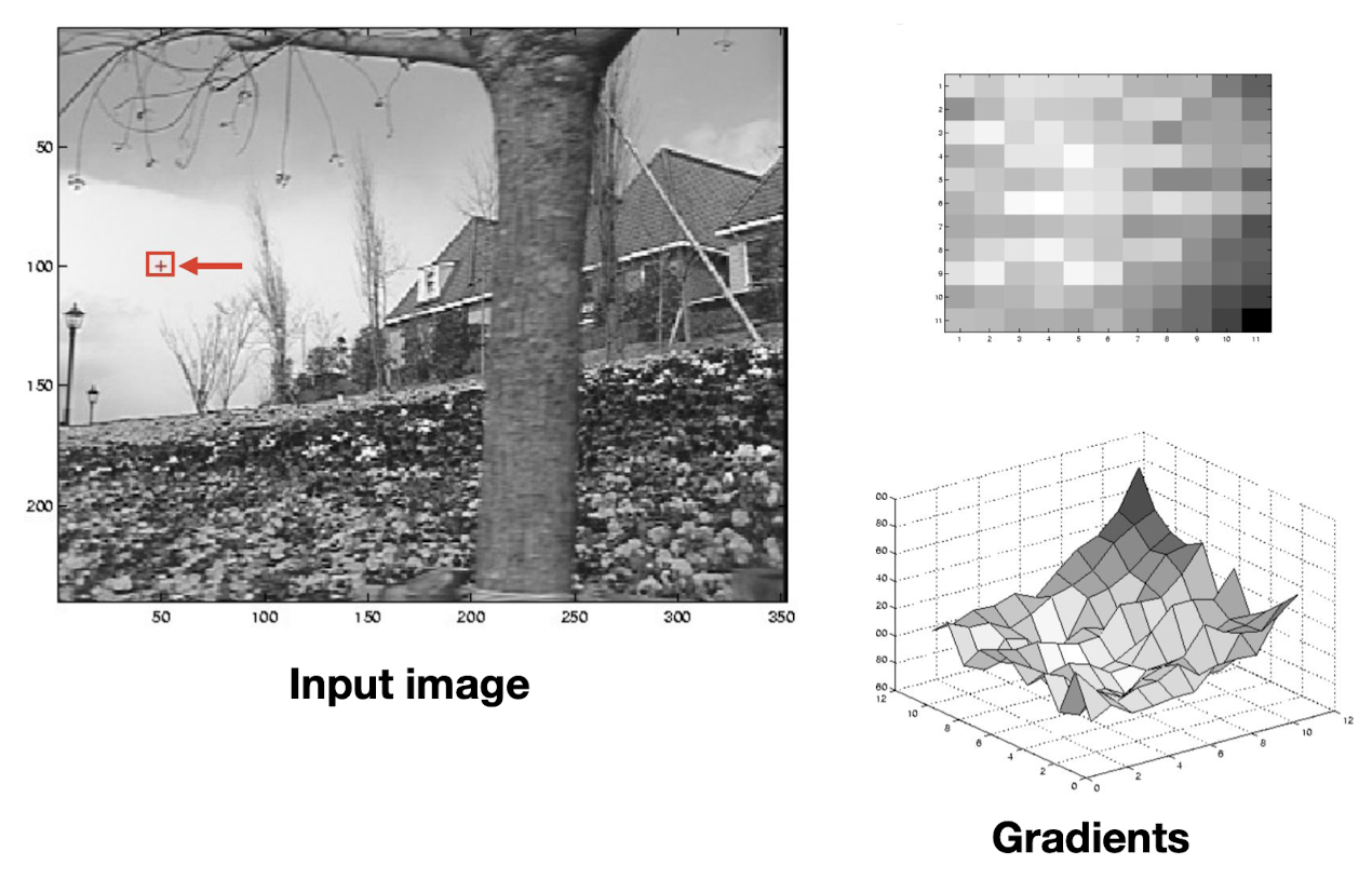
$\mathbf{Fig\ 7.}$ Low texture region (small eigenvalues case)

In case of edge, only gradient with orthogonal orientation against the edge will have large values, so that $A^\top A$ may be ill-conditioned:

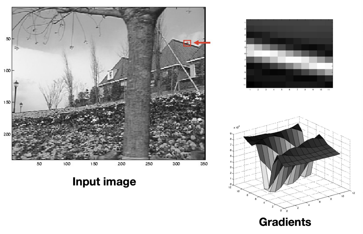
$\mathbf{Fig\ 8.}$ Edge (ill-conditioned case)

And as we expect, high textured regions such as corners will have large gradients for both directions, hence both eigenvalues will be large:

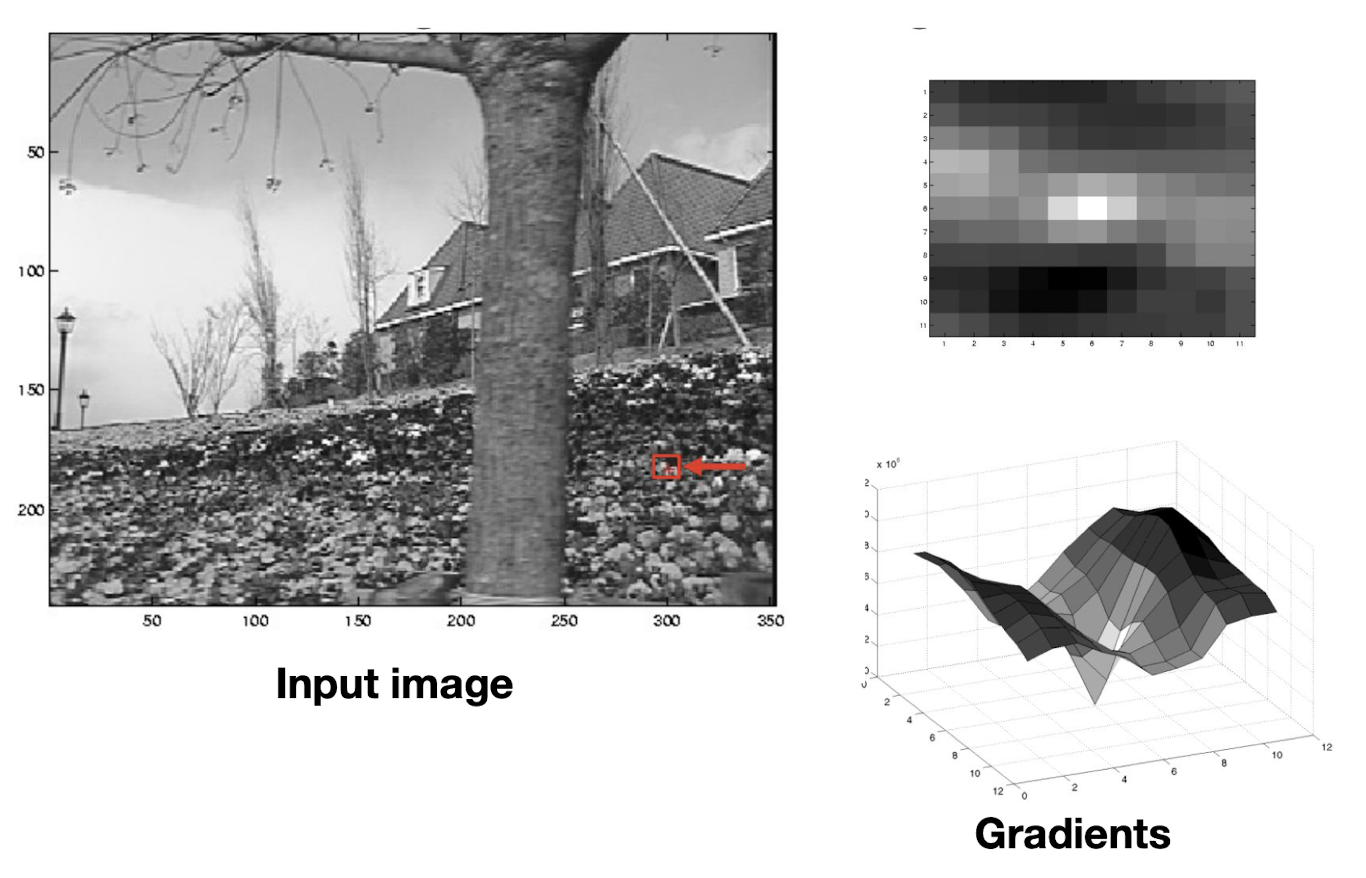
$\mathbf{Fig\ 9.}$ High textured region (best case)

And the following figure shows my own result of Lucas-Kanade algorithm:

$\mathbf{Fig\ 10.}$ An example of result of Lucas-Kanade method

Implication

If you closely look at the conformation of $A^\top A$, you may find that it has a configuration in common with Harris corner detection.

\[\begin{aligned} \underbrace{A^\top A = \left[\begin{array}{cc} \sum I_x I_x & \sum I_x I_y \\ \sum I_x I_y & \sum I_y I_y \end{array}\right]}_{\text{Lucas-Kanade}}, \quad \underbrace{M=\sum_{x, y} w(x, y) \cdot \left[\begin{array}{cc} I_x^2 & I_x I_y \\ I_x I_y & I_y^2 \end{array}\right]=V\left[\begin{array}{cc} \lambda_1 & 0 \\ 0 & \lambda_2 \end{array}\right] V^{\mathrm{T}}}_{\text{Harris Corner Detection}} \end{aligned}\]

This similarity implies that corners are good places to compute optical flow. Recall that corners have both large eigenvalues $\lambda_1, \lambda_2$ in Harris corner detection, and it is also the best condition to estimate the motion vector. It is somewhat obvious, since corners are areas with at least two different orientations of gradient, so that it does not suffer from aperture problem.

Limitation

Obviously, Lucas-Kanade method is not a perfect solution since we made a few assumptions in the formulation of algorithm which may fails in some counterexamples.

The representative failures of Lucas-Kanade method are outlined below:

• Point doesn’t move with neighbors
  • e.g. boundary of object
• Brightness constancy isn’t always true
  • e.g. deluminating changes such as bulb
  • solution. use color-invariant feature (e.g. SIFT)
• Taylor series is bad approximation when motion is very large
  • solution. compute motion in multiple image resolutions

Reference

[1] Szeliski, Richard. Computer vision: algorithms and applications. Springer Nature, 2022.
[2] A tutorial on Motion Estimation with Optical Flow with Python Implementation
[3] Wikipedia, Optical Flow
[4] Pennsylvania State University, CSE/EE486 Introduction to Computer Vision, Fall 2007