[CV] Visual Object Tracking

The objective of visual object tracking is to locate the object in a video. Throughout the time axis, the target of object is annotated at the first frame with the bounding box and then we should locate this target object for the rest of the frame:

$\mathbf{Fig\ 1.}$ Objective of Visual object tracking

There are two sub-categories of object tracking:

• Single target tracking
  • Tracking only one object in a video
  • Single-class classification (target v.s. distractor classes)
• Multi target tracking
  • Tracking multiple objects in a video
  • Mutliple-class classification (target 1, 2, 3, $\dots$ v.s. distractor classes)
    

And this is an example of object tracking in action. Despite it is the example of the multi-object case but we will focus on the single object tracking in this post.

---

Visual Object Tracking

We will formally define the problem as follows:

• Objective: locateing the object(s) over time in a video
  
• Definition: Given an object state at the initial frame $\mathbf{z}_0 = (x_0, y_0, w_0, h_0)$, identify \(\mathbf{z}_{1 : T} = \{ \mathbf{z}_1, \dots \mathbf{z}_T \}\) over a video of length $T$
  

We represent the bounding box of the object with the latent variable $\mathbf{z}$, identified by the four variables: the center location $(x, y)$ and the size of the bounding box $(w, h)$.

And as a deep learning perspective, we can consider this problem as

• Classification problem with a single object class
  
• The ground truth is given at only the initial frame
  
• Also, it may requires online learning to adapt the variations of objects or scenes in a video
  • and it must be driven by a self-supervision aspect.
    

Two Approaches in Single Object Tracking

In the case of the single object tracking, we have two different classes of solution.

One possible way is the probabilistic tracking. In probabilistic tracking, we basically model the problem of the tracking as a probabilistic inference.

When we observe the frame, we define the probabilities over possible bounding box representations. And given a probability of the initial target location, we propagate it over the remaining frames.

$\mathbf{Fig\ 2.}$ Probabilistic tracking (source Isard and Blake, 1998)

The other way is called discriminative tracking. It just formulate the object tracking as a sequential binary classification (object detection) model.

Probabilistic tracking

Probabilistic tracking methods formulate the information of the tracked object as a probability density function, and it is recursively updated with new observations arrived.

And in this approach, one of the most iconic works is particle filtering, or equivalently condensation algorithm, Sequential Monte Carlo (SMC) methods.

Suppose we have a small target template that contains a person riding a bike and the entire scene is hidden. Without any observation, our belief may be that the target object is likely to be located on the bottom side of the image.

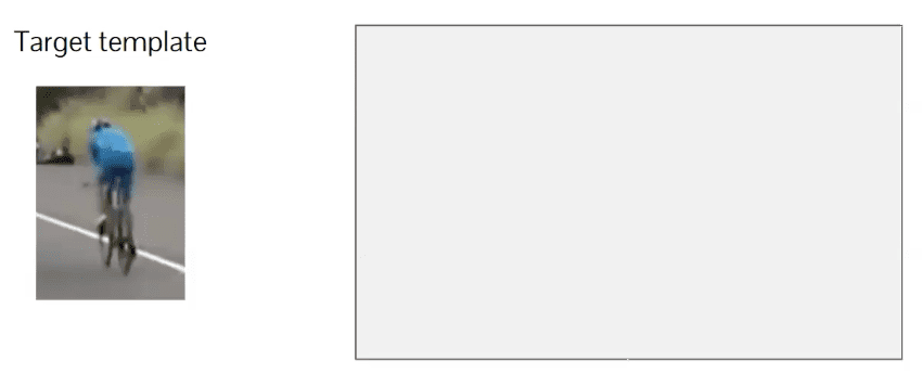
$\mathbf{Fig\ 3.}$ Without any observation

Then after witnessing the full, or some parts of the scene, we may change our mind or hold our ground.

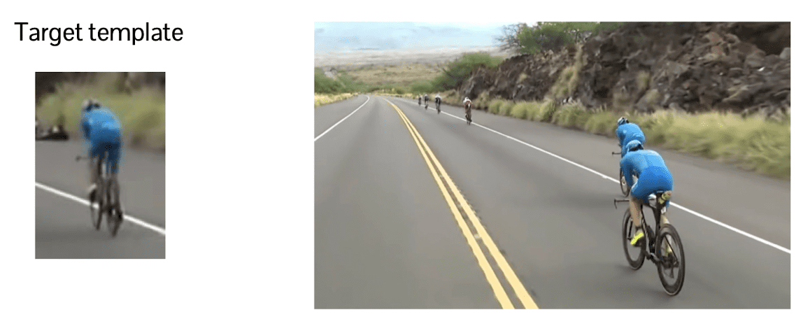
$\mathbf{Fig\ 4.}$ After observation

This high-level idea can be realized by Bayes Theorem:

• Prior $p(z)$: Where is the target likely to exist?
  
• Likelihood $p(x | z)$
  • how likely the observation coincide with the given state
  • Which region of image look similar to the target?
• Posterior $p(z | x)$
  • probability of object state given an observation
  • Where is the object in this frame?

\[\begin{aligned} p(z | x) = p(x | z)p(z) \end{aligned}\]

And, it is obviously extended to the multi-frame formulation by

\[\begin{aligned} p(\mathbf{z}_{1:T} | \mathbf{x}_{1:T}) = p(\mathbf{x}_{1:T} | \mathbf{z}_{1:T})p(\mathbf{z}_{1:T}) \end{aligned}\]

The next challenge is computation, as our goal is to estimate the entire state over the entire video frame \(\mathbf{z}_{1:T}\) at once. To make the problem easier, one possible intuitive assumption is Markov assumption:

\[\begin{aligned} & p(\mathbf{z}_t | \mathbf{z}_{1: t-1}) = p( \mathbf{z}_t | \mathbf{z}_{t-1}) \\ & p(\mathbf{x}_t | \mathbf{z}_{1: t}) = p( \mathbf{x}_t | \mathbf{z}_{t}) \end{aligned}\]

And due to the existence of latent variable $\mathbf{z}$ behind the observation $\mathbf{x}$, the dependency between variables can be visualized by Hidden Markov Model:

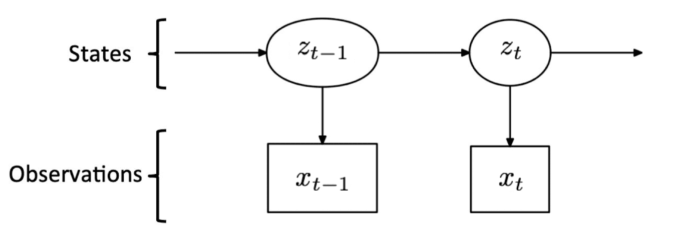
$\mathbf{Fig\ 5.}$ Our hidden Markov model

Then, based on this assumption, let’s calculate the posterior:

\[\begin{aligned} p\left(\mathbf{z}_t \mid \mathbf{x}_{1: t}\right) & \propto \color{blue}{\underbrace{\color{black}{p\left(\mathbf{x}_t \mid \mathbf{z}_t\right)}}_{\color{blue}{\text{Likelihood}}}} \color{blue}{\underbrace{\color{black}{p\left(z_t \mid \mathbf{x}_{1: t-1}\right)}}_{\color{blue}{\text{Prior}}}} \\ & = \color{blue}{\underbrace{\color{black}{p\left(\mathbf{x}_t \mid \mathbf{z}_t\right)}}_{\color{blue}{\text{Likelihood}}}} \color{red}{\underset{\text{Integration over all object locations!}}{\boxed{\color{black}{\int p\left(\mathbf{z}_t \mid \mathbf{z}_{t-1}\right) p\left(\mathbf{z}_{t-1} \mid \mathbf{x}_{1: t-1}\right) d \mathbf{z}_{t-1}}}}} \end{aligned}\]

Here, the second term of the bottom line is for the transition model that corresponds to the dynamics of the object. For example, if we know the velocity or acceleration of the object and the state of current scene, we can predict the location of object in the next frame.

And notice that \(p(\mathbf{z}_t \mid \mathbf{x}_{1:t})\) is emerging recursively. Hence, this formula recursively propagates the posterior from the previous frame to the current time step by the transition model and likelihood.

To approximate the integration, we exploit Monte Carlo approximation:

\[\begin{aligned} p\left(\mathbf{z}_t \mid \mathbf{x}_{1: t}\right) & \propto p\left(\mathbf{x}_t \mid \mathbf{z}_t\right) \int p\left(\mathbf{z}_t \mid \mathbf{z}_{t-1}\right) p\left(\mathbf{z}_{t-1} \mid \mathbf{x}_{1: t-1}\right) d \mathbf{z}_{t-1} \\ & = p(\mathbf{x}_t \mid \mathbf{z}_t) \cdot \mathbb{E}_{z_{t-1} \sim p(\; \cdot \; \mid \; \mathbf{x}_{1:t-1})} \left[ p(\mathbf{z}_t \mid \mathbf{z}_{t-1}) \right] \\ & \approx p(\mathbf{x}_t \mid \mathbf{z}_t) \sum_{i=1}^N p(\mathbf{z}_t \mid \mathbf{z}^{(i)}_{t-1}) \quad \text{ where } \quad \mathbf{z}^{(i)}_{t-1} \sim p(\mathbf{z}_{t-1} | \mathbf{x}_{1:t-1}) \end{aligned}\]

Hence, this formula can be interpreted as a propagation of the previous probability to the current time step. Given the samples from the previous distribution, it moves the sample according to transition model \(p(\mathbf{z}_t \mid \mathbf{z}_{t-1})\) and then reweight using the likelihood \(p(\mathbf{x}_t \mid \mathbf{z}_t)\). And this procedure is referred to as particle filtering, or sequential Markov-Chain Monte-Carlo since it approximates the prior distribution by MCMC sampling:

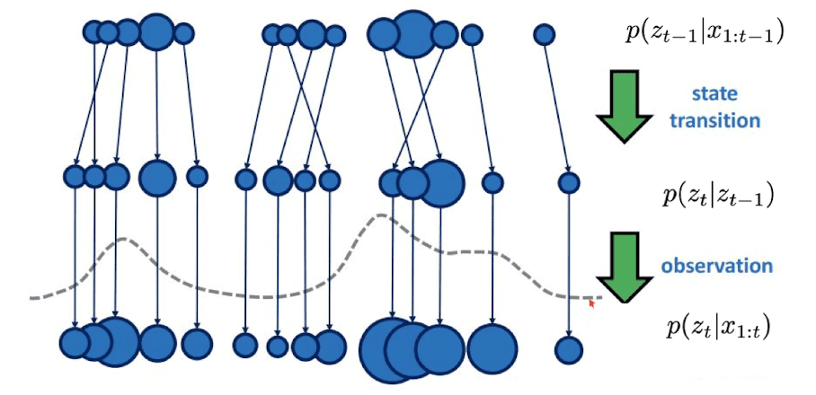
$\mathbf{Fig\ 6.}$ Particle Filtering, Sequential MCMC

In the visualization, the samples are denoted by circles and the weight of each sample is represented by the size of the circle.

Let’s apply this idea into the real problem. In the high level, the posterior distribution indicates the probability of possible bounding boxes. In the bottom figure, the distribution of target space is denoted by heat map (red is the highest) and samples are denoted by white crosses in the heat map and orange dotted box in the frame:

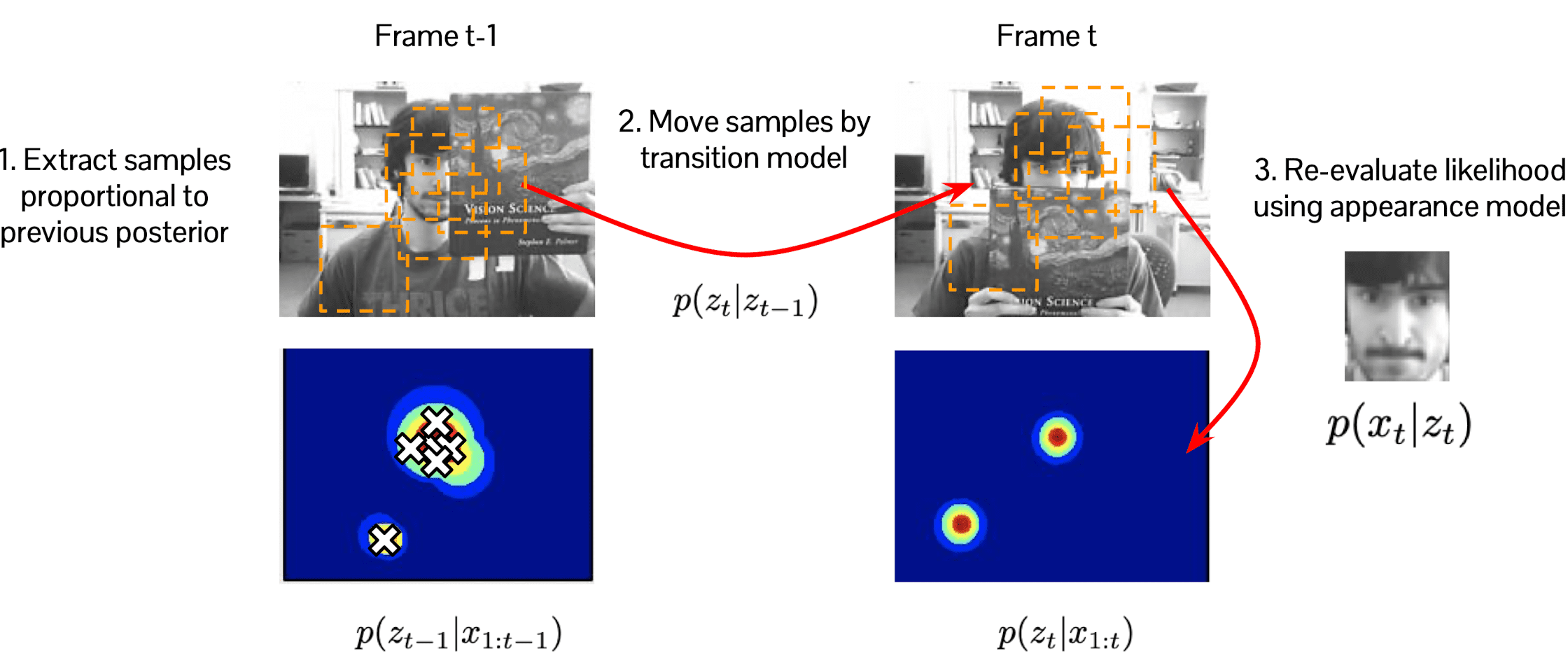
$\mathbf{Fig\ 7.}$ Particle filtering pipeline

In short, the procedure of particle filtering is outlined as below.

• Sample target states near the previous target location
• Evaluate the likelihood based on appearance model
• Select the most probable sample as the target at the current frame
• Update the target appearance model using the current tracking results

Discriminative Tracking

Discriminative tracking is intrinsically the detection problem where the classes are on the two: the foreground and the background. Since it involves a object detector that is applied to all image frames, it is equivalently referred to as tracking-by-detection paradigm.

$\mathbf{Fig\ 8.}$ Discriminative tracking framework overview

Thus once we have this kind of classifier, when the new frame is given we can randomly sample the bounding boxes around the object and then apply the classifier. A various sort of classifier, including SVM, decision tree [3], is possible to be employed as a classifier. But in this post, we will focus on ridge regression that admits a simple closed-form solution as a brief introduction of deterministic tracking:

\[f(\mathbf{w}) = \underset{\mathbf{w}}{\text{arg min }} \| \mathbf{y} - \mathbf{X} \mathbf{w} \|_2^2 + \lambda \| \mathbf{w} \|_2^2\]

where $\mathbf{y}$ denotes training labels and $\mathbf{X}$ is training data. As the objective is convex function, we have one global optimum at $\frac{\partial f(\mathbf{w})}{\partial \mathbf{w}} = 0$, i.e. $\mathbf{w}^* (\mathbf{X}^\top \mathbf{X} + \lambda I)^{-1} \mathbf{X}^\top \mathbf{y}$.

But the problem is that this computation, especially inverse computation is often very expensive for online training as we should update this classifier for every frames.

However, it turned out that it can be extremely fast if we construct positive and the negative data in a specific way. We’re going to consider that the actual object that is perfectly aligned with the bounding box as base sample, and any misaligned will be the negative samples:

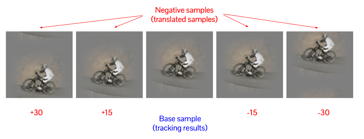
$\mathbf{Fig\ 9.}$ Examples of vertical cyclic shifts of a base sample

Let the size of the frame be $H \times W$. Then, we consider base sample $\mathbf{x}$ as $n$-dimensional array $\mathbf{x} = [x_1, x_2, \cdots, x_n]$ where $n = H * W$, i.e. flattened. Then we create data matrix $\mathbf{X}$ as a circulant matrix:

\[\begin{aligned} X=C(\mathbf{x})=\left[\begin{array}{ccccc} x_1 & x_2 & x_3 & \cdots & x_n \\ x_n & x_1 & x_2 & \cdots & x_{n-1} \\ x_{n-1} & x_n & x_1 & \cdots & x_{n-2} \\ \vdots & \vdots & \vdots & \ddots & \vdots \\ x_2 & x_3 & x_4 & \cdots & x_1 \end{array}\right] \end{aligned}\]

thus only the first row will be positive sample. From the mathematical fact that any circulant matrices can be made diagonal by Discrete Fourier Transform (DFT), it can be written as

\[\begin{aligned} \mathbf{X} = F^\top \text{diag} (\widehat{\mathbf{x}}) F \quad \text{ where } \quad F^\top F = I \end{aligned}\]

where $F$ is a constant matrix known as the DFT matrix, which is the unique matrix that computes the DFT of any input vector as $\mathcal{F}(\mathbf{z}) = \sqrt{n} F \mathbf{z}$ and does not depend on $\mathbf{x}$. $\widehat{\mathbf{x}}$ denotes the DFT of the generating vector $\mathbf{x}$ of circulant matrix $\mathbf{X}$, i.e. $\widehat{\mathbf{x}} = \mathcal{F} (x)$.

The most important aspect of diagonalizability is that the computation speed of operations is extremely rapid. For example, matrix inner product of diagonalizable matrix can be obtained by Hardamard product \(\mathbf{X}^\top \mathbf{X} = F^\top \text{diag} (\widehat{\mathbf{x}} \odot \widehat{\mathbf{x}})\). Then, our solution is now much efficient to compute:

\[\begin{aligned} \mathbf{w}^* & = (\mathbf{X}^\top \mathbf{X} + \lambda I)^{-1} \mathbf{X}^\top \mathbf{y} \\ & = \text{diag} \left( \frac{\widehat{\mathbf{x}}^*}{\widehat{\mathbf{x}}^* \odot \widehat{\mathbf{x}} + \lambda \cdot \mathbf{1}} \right) \mathbf{y} \end{aligned}\]

Furthermore, we extend the formula to kernelized version:

\[\begin{aligned} \mathbf{w}^* & = (K + \lambda I)^{-1} \mathbf{X}^\top \widehat{\mathbf{y}} \end{aligned}\]

hence it can be also computed efficiently if kernel matrix $K$ is circulant matrix. And [3] shows that most useful kernel matrices such as Gaussian, linear and polynomial kernels, etc. are circulant.

Challenges: Appearance Modeling

Thus far, we focus on the way how we track or detect the object through the time. Another challenges in classical approaches is to model severe appearance variations due to to geometric changes (e.g. pose, arEculaEon, scale) or photometric factors (e.g. illumination, appearance) in a video, which modeling is called appearance modeling.

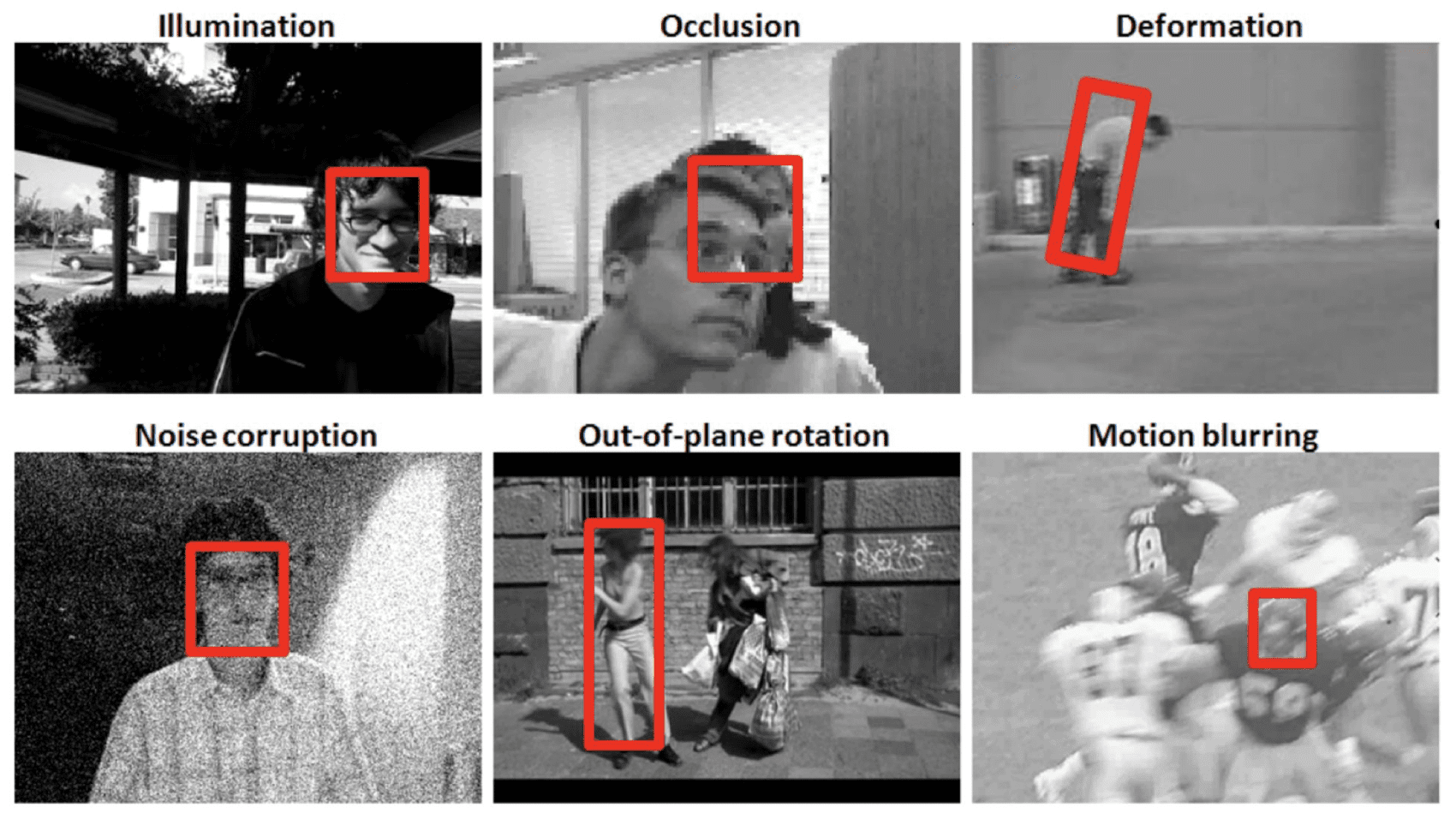
$\mathbf{Fig\ 10.}$ Illustration of complicated appearance changes in visual object tracking (source: [4])

Hence in terms of the appearance modeling, researchers have tried to propose robust appearance descriptors such as color histogram, key-points like corners, SIFT, etc. But we already know the issue of the hand design features: it is prone to overfitting and not generalizable to a wide range of appearances.

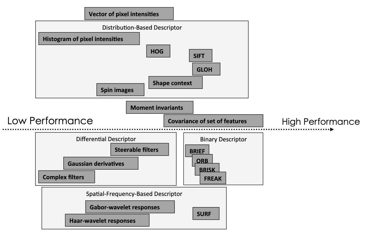
$\mathbf{Fig\ 11.}$ Bulk of hand-designed features
(source: Mikolajczyk et. al. "A performance evaluation of local descriptors." PAMI 2005)

As a result, it was natural that the trend was shifted onto deep learning, likewise other areas of computer vision have underwent.

Hong, Seunghoon, et al. directly applied pretrained CNN for object tracking as a feature to classify by SVM, but following the traditional pipeline of discriminative tracking:

$\mathbf{Fig\ 12.}$ Application of Pretrained CNN feature for visual object tracking (source: [5])

And not suprisingly, it achieved the state-of-the-art tracking algorithms compared to classical approaches:

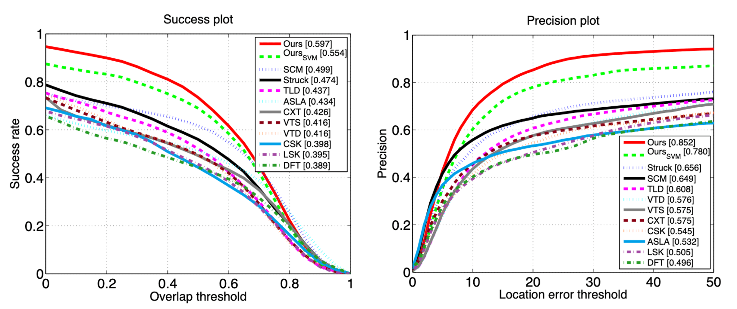
$\mathbf{Fig\ 13.}$ Average success plot (left) and precision plot (right) (source: [5])

Over and above that, Multi-Domain Network (MDNet) won the VOT2015 Challenge by exploiting end-to-end aspect of deep learning. It employs the standard architecture of CNN classifier (CNN feature extractor + Fully-connected classifier). But one different thing is it separated classification heads for each video, i.e. $N$ number of classification heads for $N$ videos, since the definition of foreground and background are different for each video.

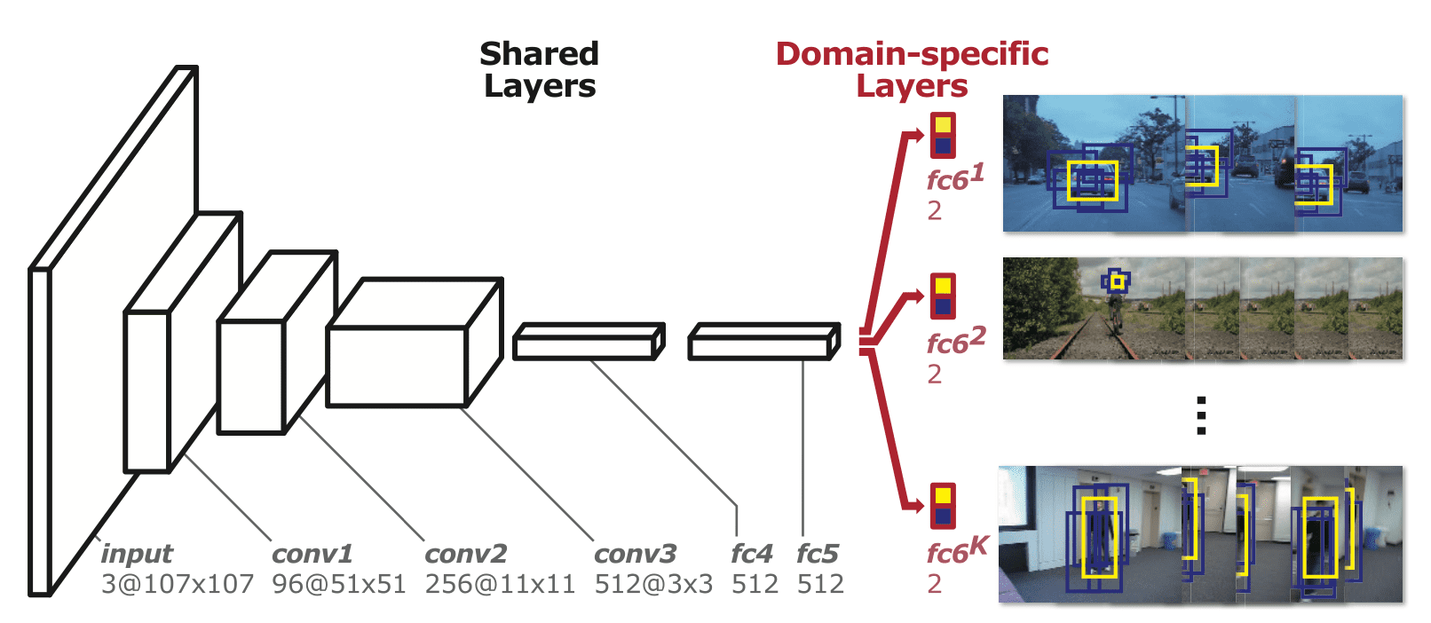
$\mathbf{Fig\ 14.}$ The architecture of our Multi-Domain Network (source: [6])

And in the next post, we will discuss about more advanced CNNs for visual object tracking deeper.

Reference

[1] Stanford University CS231B: The Cutting Edge of Computer Vision, Spring 2015
[2] Isard, Michael, and Andrew Blake. “Condensation—conditional density propagation for visual tracking.” International journal of computer vision 29.1 (1998): 5-28.
[3] Henriques, João F., et al. “High-speed tracking with kernelized correlation filters.” IEEE transactions on pattern analysis and machine intelligence 37.3 (2014): 583-596.
[4] Li, Xi, et al. “A survey of appearance models in visual object tracking.” ACM transactions on Intelligent Systems and Technology (TIST) 4.4 (2013): 1-48.
[5] Hong, Seunghoon, et al. “Online tracking by learning discriminative saliency map with convolutional neural network.” International conference on machine learning. PMLR, 2015.
[6] Nam, Hyeonseob, and Bohyung Han. “Learning multi-domain convolutional neural networks for visual tracking.” Proceedings of the IEEE conference on computer vision and pattern recognition. 2016.