[CV] Transformers in Vision

Introduction

Transformer-based models have become the fundametal model of LLMs and exhibited remarkable performance in NLP. Popular examples include BERT, the GPT family, and RoBERTa. Due to Transformers’ computational efficiency and scalability, it has become possible to train models of unprecedented size, with over 100B parameters. For instance, while the BERT-large model with 340M parameters showcased significant capability, it was notably surpassed by the GPT-3 model with 175B parameters. Moreover, the latest Switch transformer achieves an unprecedented scale of 1.6T parameters.

In this regime, extending the Transformer paradigm to computer vision is a natural progression. Although images have distinctive structure such as spatial/temporal coherence, necessitating innovative strategies, Transformer models have proven successful in various computer vision tasks, including image recognition, object detection, segmentation, image generation, etc. This post introduces Transformer-based visual foundation models that accelerate the evolution from CNNs to Transformers.

Vision Transformer (ViT)

1. 2D Image to Patch Embeddings
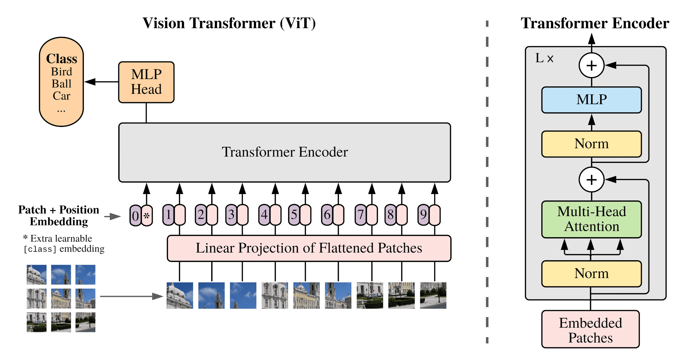
   Recall that the Transformer receives as input a 1D sequence of token embeddings. To handle 2D images, ViT reshape the image $\mathbf{x} \in \mathbb{R}^{H \times W \times C}$ into a sequence of flattened 2D patches $\mathbf{x}_p \in \mathbb{R}^{N \times (P^2 \cdot C)}$, where $(H, W)$ is the resolution of the original image, $C$ is the number of channels, $(P, P)$ is the resolution of each image patch, and $N = H \cdot W/P^2$ is the resulting number of patches, which also serves as the effective input sequence length for the Transformer. Then the patches are flattened and mapped to $D$ dimensional patch embeddings with a trainable linear projection. Similar to BERT’s [CLS] token, it prepends a learnable embedding to the sequence of embedded patches ($\mathbf{z}_0^0 = \mathbf{x}_{\mathrm{class}}$). Also, learnable 1D position embeddings $\mathbb{E}_{\mathrm{pos}}$ are added to the patch embeddings to retain positional information. (The authors have not observed significant performance gains from using more advanced embeddings.) $$ \begin{aligned} \mathbf{z}_0 & =\left[\mathbf{x}_{\text {class }} ; \mathbf{x}_p^1 \mathbf{E} ; \; \mathbf{x}_p^2 \mathbf{E} ; \; \cdots ; \; \mathbf{x}_p^N \mathbf{E}\right]+\mathbf{E}_{pos} \quad \text{ where } \mathbf{E} \in \mathbb{R}^{\left(P^2 \cdot C\right) \times D}, \mathbf{E}_{p o s} \in \mathbb{R}^{(N+1) \times D} \end{aligned} $$ The following figure visualizes the learned embeddings. We can observe that the top principal components of the learned embedding filters $\mathbf{E}$ resemble basis functions for a low-dimensional representation of the fine structure within each patch. Also, the positional embeddings learn to capture spatial distances within the image in terms of the similarity, i.e. closer patches tend to have more similar position embeddings.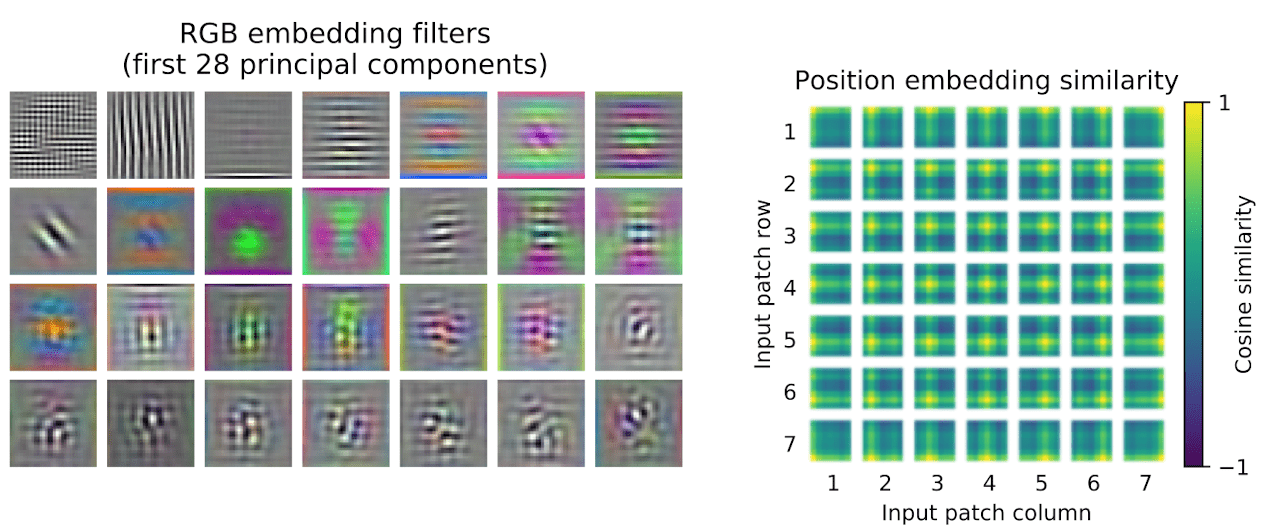

   

   $\mathbf{Fig\ 1.}$ (Left) Filters of the initial linear embedding. (Right) Similarity of position embeddings. (Kolesnikov et al. 2021)

2. Alternating layers of multiheaded self-attention and MLP blocks
   For each element in an input sequence $\mathbf{z} \in \mathbb{R}^{N \times D}$, the attention weights $A_{ij}$ and the resulting value of self-attention can be computed by $$ \begin{aligned} {[\mathbf{q}, \mathbf{k}, \mathbf{v}]} & = \mathbf{z} \mathbf{U}_{q k v} & \mathbf{U}_{q k v} \in \mathbb{R}^{D \times 3 D_h} \\ A & = \operatorname{softmax}\left(\mathbf{q k}^{\top} / \sqrt{D_h}\right) & A \in \mathbb{R}^{N \times N} \\ \operatorname{SA}(\mathbf{z}) & = A \mathbf{v} \end{aligned} $$ Multihead Self-Attention is an extension of SA in which we run $k$ self-attention operations, called “heads” and project their concatenated outputs. To keep compute and number of parameters constant when changing $k$, we set $D_h = D/k$. $$ \begin{aligned} \operatorname{MSA}(\mathbf{z}) = \left[\operatorname{SA}_1(\mathbf{z}) ; \operatorname{SA}_2(\mathbf{z}) ; \; \cdots ; \; \operatorname{SA}_k(\mathbf{z}) \right] \mathbf{U}_{msa} \quad \mathbf{U}_{msa} \in \mathbb{R}^{k \cdot D_h \times D} \end{aligned} $$ Then, we apply MLP block that contains two layers with a GELU non-linearity to the output of MSA. Layer Normalization is applied before every block, and residual connections after every block. Formally, $$ \begin{aligned} \mathbf{z}_{\ell}^{\prime} & =\operatorname{MSA}\left(\operatorname{LN}\left(\mathbf{z}_{\ell-1}\right)\right)+\mathbf{z}_{\ell-1}, & & \ell=1 \ldots L \\ \mathbf{z}_{\ell} & =\operatorname{MLP}\left(\operatorname{LN}\left(\mathbf{z}_{\ell}^{\prime}\right)\right)+\mathbf{z}_{\ell}^{\prime}, & & \ell=1 \ldots L \\ \end{aligned} $$ And the state at the output of the Transformer encoder $\mathbf{z}_L^0$ serves as the image representation $\mathbf{y} = \operatorname{LN}(\mathbf{z}_L^0)$. Similar to BERT, both during pre-training and fine-tuning, a classification head is attached to $\mathbf{z}_L^0$.

At fine-tuning stage, the resolution may be higher than pre-training dataset. In this case, the pre-trained position embeddings may no longer be meaningful. We therefore perform 2D interpolation of the pre-trained position embeddings, according to their location in the original image. See $\mathbf{Fig\ 2.}$ for the overall architecture of ViT.

$\mathbf{Fig\ 2.}$ ViT Overview (Kolesnikov et al. 2021)

ViT exhibits significantly reduced image-specific inductive bias compared to CNNs. In CNNs, attributes such as locality, two-dimensional neighborhood structure, and translation equivariance are inherent at each layer throughout the entire model. In contrast, ViT confines the locality and translational equivariance aspects to MLP layers, while self-attention layers operate globally. The utilization of two-dimensional neighborhood structure is minimal, manually injected by dividing the image into patches and during fine-tuning to adjust position embeddings for varying image resolutions.

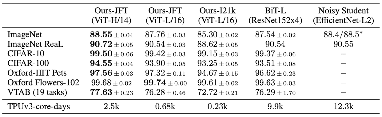
When pre-trained on large amounts of data and transferred to multiple mid-sized or small image recognition benchmarks (ImageNet, CIFAR-100, VTAB, etc.), ViT attains excellent outcomes in comparison to SOTA CNNs, demanding significantly diminished computational resources for training.

$\mathbf{Fig\ 3.}$ Comparison with SOTA on popular image classification benchmarks (Kolesnikov et al. 2021)

$\mathbf{Fig\ 4.}$ (Left) Trasfer to ImageNet (Right) Linear few-shot evaluation on ImageNet (Kolesnikov et al. 2021)

$\mathbf{Fig\ 5.}$ Scaling study: Performance v.s. pre-training compute.
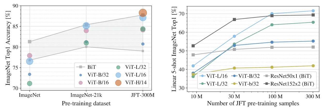
ViT generally outperforms ResNets with the same computational budget. (Kolesnikov et al. 2021)

Swin Transformer

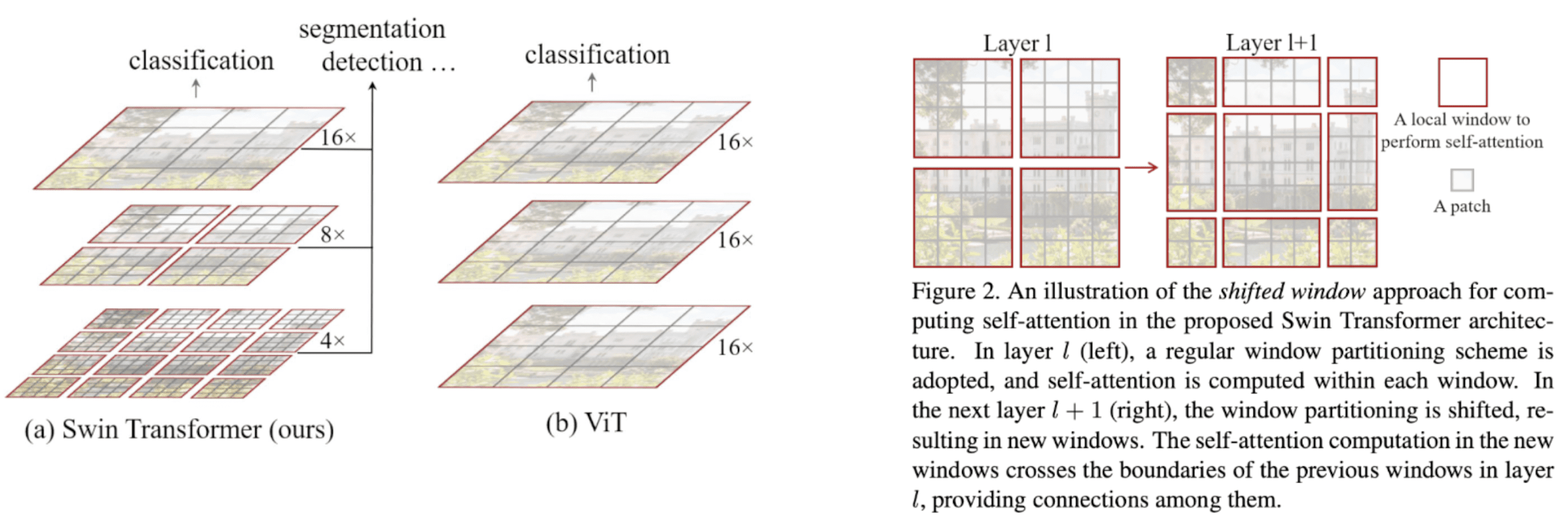
ViT partitions the 2D $H \times W$ image into $H \cdot W / P^2$ number of patches with the fixed resolution $P \times P$, which is problematic in visual domain that the scale of visual elements is critical to image perception. For specific example, imagine the semantic segmentation and object detection tasks in computer vision. As varying receptive field of CNNs is the longstanding problem in various vision tasks, Liu et al. ICCV 2021 also tackles these issues in ViT, proposing a hierarchical Transformer called Swin Transformer whose representation is computed with Shifted windows.

$\mathbf{Fig\ 6.}$ Patches in multiple resolutions and Shifted window approach of Swin Transformer (Liu et al. 2021)

The main differences with ViT are summarized below.

1. Patch Processing
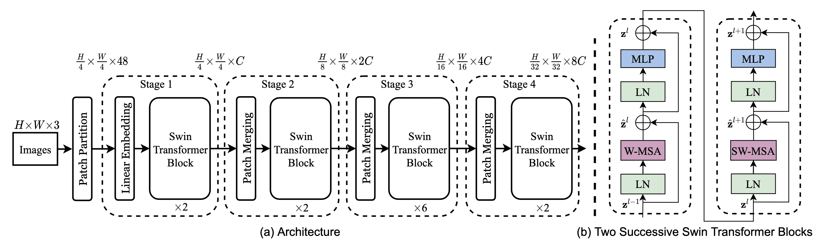
   The Swin Transformer constructs a hierarchical representation by starting from small-sized patches (tokens) and gradually mergin neighboring patches in deeper Transformer layers. It has total 4 stages for patch resolutions: $4 \times 4$, $8 \times 8$, $16 \times 16$, and $32 \times 32$. (See the left of $\mathbf{Fig\ 6.}$) After each stage, the number of tokens is reduced by patch merging layers to produce a hierarchical representation. It concatenates the features of each group of $2 \times 2$ neighboring patches, hence reducing the nmber of tokens by $4$, and applies a linear layer on the concatenated features.
   
   With theses hierarchical feature maps, the Swin Transformer can leverage advanced techniques such as feature pyramid networks or U-Net.


2. Shifted Window-based Self-Attention
   The global self-attention in the standard Transformer and ViT results in quadratic complexity, making it impractical for numerous vision problems that demand an extensive set of patches for dense prediction or to represent a high-resolution image. To overcome this issue, the Swin Transformer compute self-attention within non-overlapping local windows. The size of window $M$ is considered as a hyperparameter.
   
   Simple window-based self-attention lacks connections across windows. To construct cross-window connections with efficient complexity, the paper propose a shifted non-overlapped window partitioning. Consider two consecutive Transformer blocks. The first block uses a regular window partitioning and suppose that the feature map is partitioned into $M \times M$ windows. Then the next block adpots a shifted windowing configuration that is shifted from that of the preceding layer, by displacing the windows by $(\lfloor \frac{M}{2} \rfloor, \lfloor \frac{M}{2} \rfloor)$ pixels from the regularly partitioned windows. (See the right of $\mathbf{Fig\ 6.}$)
   
   Note that shifted window partitioning results in more windows, from $\lceil \frac{H}{M} \rceil \times \lceil \frac{W}{M} \rceil$ to $(\lceil \frac{H}{M} \rceil + 1) \times (\lceil \frac{W}{M} \rceil + 1)$. For efficiency, the paper leverages an efficient batch computation approach by cyclic shift (in PyTorch, torch.roll() operation) as $\mathbf{Fig\ 7.}$ illustrates. A resulting batched window may be composed of several sub-windows that are not indeed adjacent in the feature map, therefore it adds an appropriate attention mask to $QK^\top$ to discard the connections between that sub-windows. As a result, the number of batched windows remains the same as that of regular window partitioning, thus has the low latency.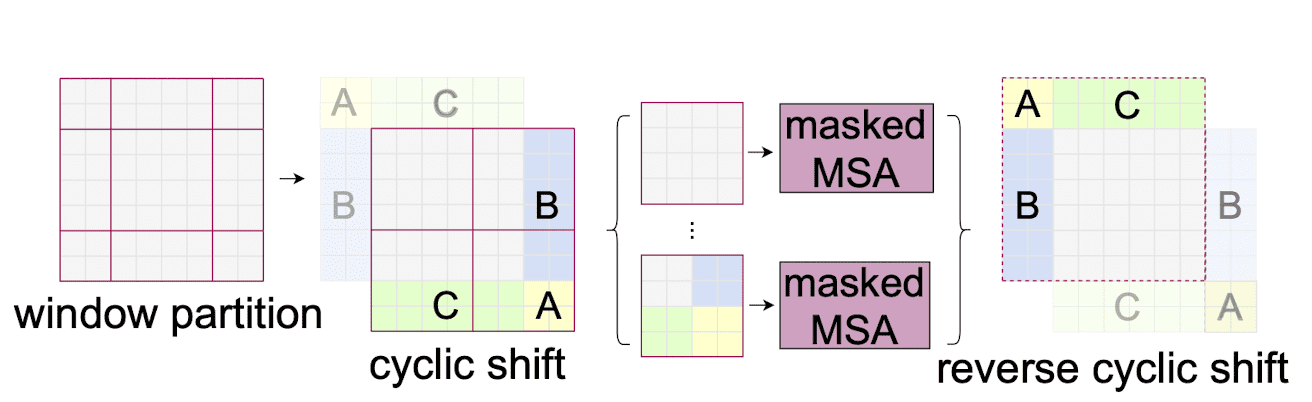

   

   $\mathbf{Fig\ 7.}$ Efficient batch computation approach (Liu et al. 2021)
   
   Then consecutive Swin Transformer blocks are computed as $$ \begin{aligned} & \hat{\mathbf{z}}^l = \textrm{W-MSA} (\mathrm{LN} (\mathbf{z}^{l-1})) + \mathbf{z}^{l-1} \\ & \mathbf{z}^l = \mathrm{MLP} (\mathrm{LN} (\hat{\mathbf{z}}^l)) + \hat{\mathbf{z}}^l \\ & \hat{\mathbf{z}}^{l+1} = \textrm{SW-MSA} (\mathrm{LN} (\mathbf{z}^l)) + \mathbf{z}^l \\ & \mathbf{z}^{l+1} = \mathrm{MLP} (\mathrm{LN} (\hat{\mathbf{z}}^{l+1})) + \hat{\mathbf{z}}^{l+1} \\ \end{aligned} $$ Furthermore, in self-attention, it leverages a relative position bias $B \in \mathbb{R}^{M^2 \times M^2}$ to each head: $$ \begin{aligned} \mathrm{Attention}(Q, K, V) = \mathrm{softmax}(QK^\top / \sqrt{d} + B) V \quad \text{ where } Q, K, V \in \mathbb{R}^{M^2 \times d} \end{aligned} $$ Since the relative position along each axis lies in the range $[- M + 1, M - 1]$, we can parameterize a smaller-size bias matrix $\hat{B} \in \mathbb{R}^{(2M - 1) \times (2M - 1)}$ and values in $B$ can be taken from $\hat{B}$. Specifically, the following figures visualize the range of relative position and why $(2M - 1) \times (2M - 1)$ number of parameters are sufficient to represent $M^2 \times M^2$ relative position bias parameters.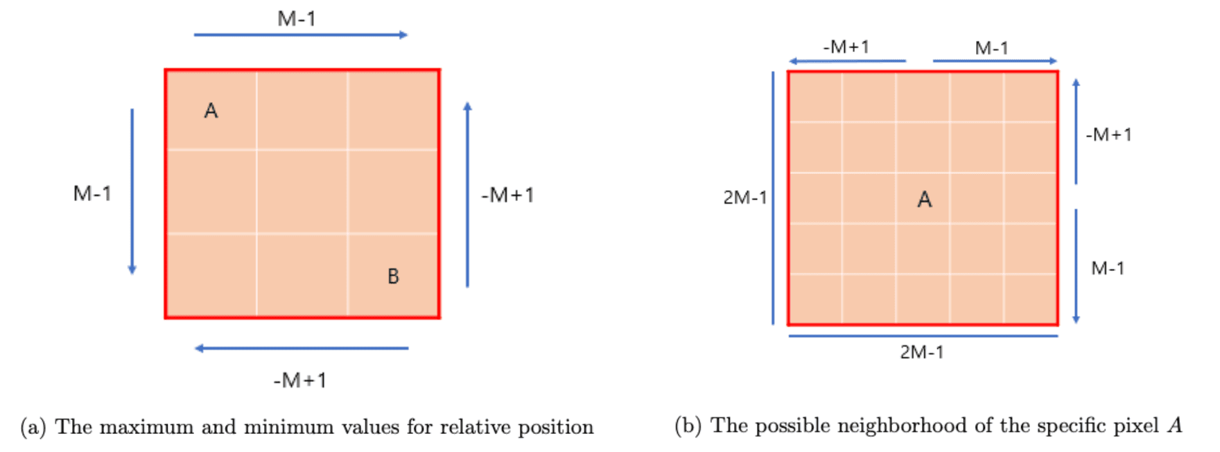

   

   $\mathbf{Fig\ 8.}$ Visualization of relative positions (blog)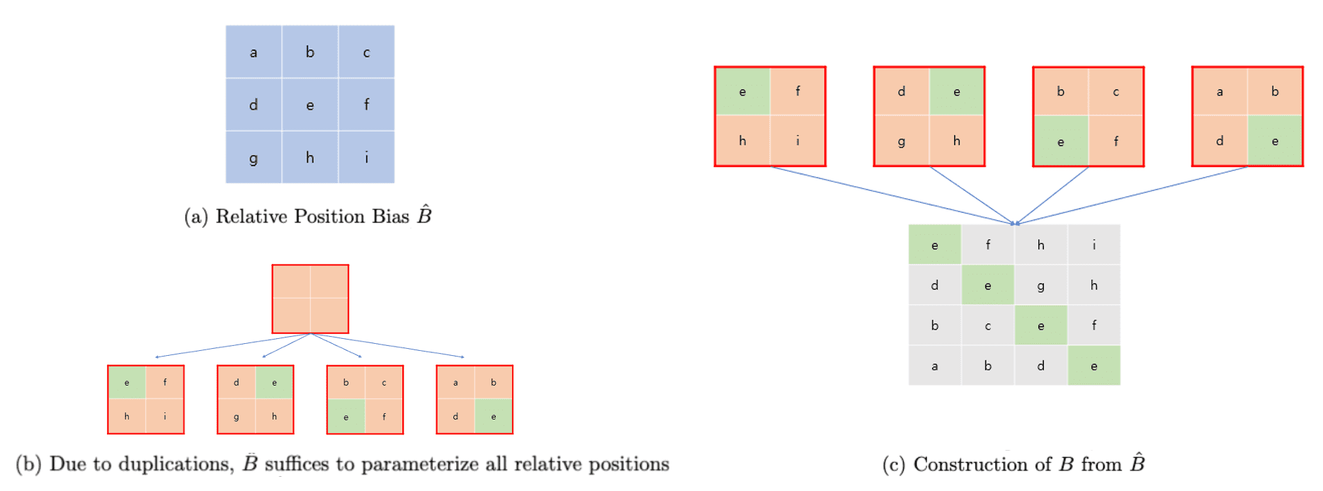

   

   $\mathbf{Fig\ 9.}$ Parameterization of $\hat{B}$ (blog)
   
   

In summary, the overall architecture of Swin Transformer is illustrated in $\mathbf{Fig\ 10.}$ Depending on the model size, the Swin Transformer is termed as Swin-T, Swin-S, Swin-B, Swin-L: $0.25 \times$, $0.5 \times$, $1 \times$, and $2 \times$ the model size and computational complexity, respectively.

• Swin-T: $C = 96$, layer numbers \(\{2, 2, 6, 2\}\)
• Swin-S: $C = 96$, layer numbers \(\{2, 2, 18, 2\}\)
• Swin-B: $C = 128$, layer numbers \(\{2, 2, 18, 2\}\)
• Swin-L: $C = 192$, layer numbers \(\{2, 2, 18, 2\}\)

$\mathbf{Fig\ 10.}$ The architecture of a Swin Transformer (Swin-T) and Blocks (Liu et al. 2021)

In image classification domain, the Swin Transformer surpasses the previous state-of-the-art architecture DeiT with comparable complexities. Additionally, it demonstrates performance comparable to the EfficientNet architectures, achieving a slightly superior speed/accuracy trade-off. Also, Swin Transformer achieves the state-of-the-art performance on COCO object detection and ADE20K semantic segmentation, significantly surpassing previous best methods. For more details and experiment results, please refer to the original paper.

$\mathbf{Fig\ 11.}$ Results on Image Classification and Ablation study on the shifted windows approach and different position embeddings.
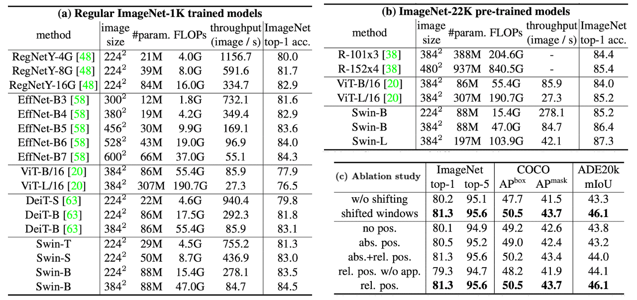
abs. pos. stands for the absolute position embedding term of ViT. (Liu et al. 2021)

Reference

[1] Kolesnikov et al. “An Image is Worth 16x16 Words: Transformers for Image Recognition at Scale”, ICLR 2021
[2] Liu et al. “Swin Transformer: Hierarchical Vision Transformer using Shifted Windows”, ICCV 2021
[3] Han Hu, “Swin Transformer supports 3-billion-parameter vision models that can train with higher-resolution images for greater task applicability”, Microsoft Research Blog, published June 21, 2022