[CV] Neural Style Transfer

Neural Style Transfer is an articifial system that blend a content from one image and a style of another image (ex. artwork by a famous painter) together, so that the output image looks like the content image, but “painted” in the style of the reference image. [4] In other words, in neural style transfer our goal is to make feature of one image look more like the features in another image, and which features are extracted from images by trained deep neural network.

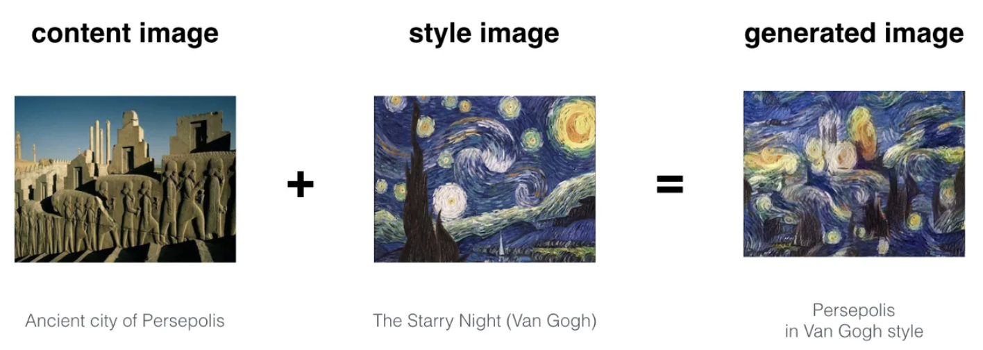
$\mathbf{Fig\ 1.}$ Neural Style Transfer (credit: blackburn)

Neural style transfer indeed refers to all algorithms of style transfer characterized by use of deep neural networks. But as it was first published in the paper “A Neural Algorithm of Artistic Style” by Leon Gatys et al. [1], [2], we will address the mechanism of neural style transfer based on this paper.

And in the community of computer vision, style transfer is usually studied as a generalization of problem of texture synthesis. (Also, the style representation of paper is following the formulation of texture synthesis) Although style is very related to texture, we may not limit concept of style to texture. Style is much more general concept than texture: it involves a large degree of simplification and shape abstraction effects including texture.

---

Algorithm overview

One main characteristic of neural style transfer is the image is generated by backpropagation, not by network like VAE or GAN. The overall training of neural style transfer is outlined below:

$\mathbf{Fig\ 2.}$ Overview of algorithm of Neural-style transfer proposed by Gatys et al. 2015 [1]

An initially random noise $\vec{x}$, content image $\vec{x}_c$ and style image $\vec{x}_s$ are feeded it through the CNN. Then we define losses \(\mathcal{L}_{\text{content}}\) and \(\mathcal{L}_{\text{style}}\) in order to dissolve both content and style into $\vec{x}$, and successively backpropagate combined total loss through the network with the CNN weights fixed in order to update the pixels of noise $\vec{x}$. After several epochs of training, we hope that $\vec{x}$ which matches the style of $\vec{x}_s$ and the content of $\vec{x}_c$ is generated.

But, to understand the algorithm the most important thing we have to discuss about is how can we quantify the content and style of the image.

Content representation

Deep convolutional neural networks for image classfication develop a representation that contains information about content of the image rather than its pixel values of image.

If we visualize the feature map of each intermediate layer of network, deeper layers capture the high-level content, while shallower layers simply contain the pixel values of the original image.

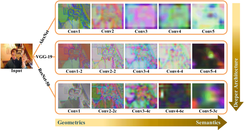
$\mathbf{Fig\ 3.}$ Visualization of feature maps from deep image classification networks (credit: Gao et al. 2020)

To put it another way, the model processes the input to high-level representations that are explicitly sensitive to the actual content of the image, but on the other hand relatively invariant to its precise pixel values, along the hierarchy of the network (due to increasing receptive field size and feature space complexity). In the figure below, for example, one can observe that deeper layers output the high-level content that do not constrain the exact pixel values of the reconstruction that much.

$\mathbf{Fig\ 4.}$ Generated images from the feature maps of deep convolutional neural network

Hence, the authors define these features as the content representation. For the next step, we need to generate $\vec{x}$ that contains similar content with $\vec{x}_c$. And by minimizing the following MSE loss, we may force $x$ to reside in the similar content space with $\vec{x}_c$:

\[\begin{aligned} \mathcal{L}_{\text{content}} = \frac{1}{2} \sum_{l = 1} \sum_{i, j, k} (P_{ijk}^l - F_{ijk}^l) \end{aligned}\]

where $P_l$ and $F_l$ are feature maps of $\vec{x}_c$ and $\vec{x}$ in layer $l$, respectively.

Style representation

Style of image is referred to as features that determines how the structure of image (content) is colored, rendered, and textured, etc. so that it allows us to display a single image in several ways.

For example, despite horse and zebra have exactly same body structures, i.e. content, they become whole another object according to the way how they textured:

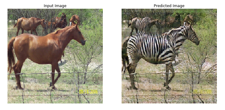
$\mathbf{Fig\ 5.}$ Horse and Zebra - Similar content but different style

A style of image is stationary in the image, i.e. has the same local properties everywhere in image. Thus in contrast to content representation, which focuses on preserving spatial locations of features, style representation should be focus on local relationship between features.

To discard the spatial information in the feature maps and take into account the localization, the authors quantified a style of image as correlation of feature maps:

\[\begin{aligned} G_{km}^l = \text{Cov}(F^l_k, F^l_m) = \sum_{i} F^l_{ki} F^l_{mi} \end{aligned}\]

where $k$ and $m$ denote the channel dimension. Hence, $G^l = \text{Cov}(F^l) \in \mathbb{R}^{N_l \times N_l}$ is our style representation, which is a Gram matrix that computes correlation of feature maps of each channel.

Finally, we force the image $\vec{x}$ to match the style of $\vec{x}_s$ by minimizing

\[\begin{aligned} E_l = \frac{1}{4N_l^2 M_l^2} \sum_{i, j} (G_{ij}^l - A_{ij}^l)^2 \end{aligned}\]

where $A^l$ is a Gram matrix that is correlation of feature map of $\vec{s}$ in layer $l$, $S^l$, and as a whole

\[\begin{aligned} \mathcal{L}_{\text{style}}(\vec{x}_s, \vec{x}) = \sum_{l} w_l E_l \end{aligned}\]

Here, $w_l$ denotes different weight on each layer and it allows to prioritize relative contribution to desired style of different levels of abstraction. As layer goes deeper, receptive field increases and feature space forms more complicately. In the aftermath of this, the model is able to capture a wider range of local relationships:

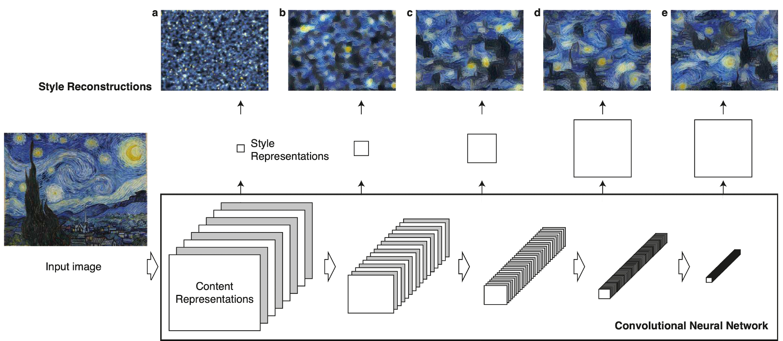
$\mathbf{Fig\ 6.}$ Multi-scale style represenation

Hence, our style representation is considered as a multi-scale representation. And matching the style up to higher layers preserves local structures a large scale, yielding to a smoother and more continuous visual result. So we contain all higher layers for reconstruction:

\[\begin{aligned} w_l = \begin{cases} 1 & l = \text{conv1_1 }, \text{conv2_1 }, \text{conv3_1 }, \text{conv4_1 }, \text{conv5_1} \\ 0 & \text{otherwise } \end{cases} \end{aligned}\]

Notably, as it was mentioned, our formulation of style of image is originally designed to capture texture information [8].

Demystifying Gram matrix

Although the use of Gram matrix is not fully and precisely explained in the original paper, Yanghao Li et al. [7] proposed mathematical grounds for Gram matrix in style transfer. The authors theoretically prove that matching the Gram matrices (minimzing $\mathcal{L}_\text{style}$) corresponds to Maximum Mean Discrepancy (MMD). Precisely, they show that

\[\begin{aligned} E_l = \mathcal{L}_{\text {style }}^l= & \frac{1}{4 N_l^2 M_l^2} \sum_{k_1=1}^{M_l} \sum_{k_2=1}^{M_l}\left(k\left(\mathbf{f}_{\cdot k_1}^l, \mathbf{f}_{\cdot k_2}^l\right)\right. \\ & \left.+k\left(\mathbf{s}_{\cdot k_1}^l, \mathbf{s}_{\cdot k_2}^l\right)-2 k\left(\mathbf{f}_{\cdot k_1}^l, \mathbf{s}_{\cdot k_2}^l\right)\right) \\ = & \frac{1}{4 N_l^2} \operatorname{MMD}^2\left[\mathcal{F}^l, \mathcal{S}^l\right] \end{aligned}\]

where $k (\mathbf{x}, \mathbf{y}) = (\mathbf{x}^\top \mathbf{y})^2$, and \(\mathbf{f}_{\cdot i}^l\) and \(\mathbf{s}_{\cdot i}^l\) are $i$-th column vector of $\mathcal{F}^l$ and $\mathcal{S}^l$, respectively.

Note that Maximum Mean Discrepancy (MMD) is a distance-measure between two probability distributions like KL-divergence.

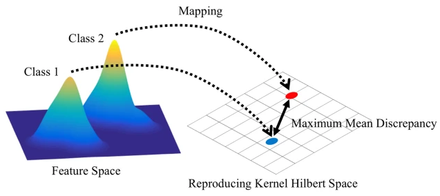
$\mathbf{Fig\ 7.}$ Maximum Mean Discrepancy (MMD)

As a result, the style of a image can be intrinsically considered as feature distributions in different layers of CNN, and the style transfer amounts to be a distribution alignment process from the content image to the style image.

Style Transfer

To transfer the style of $\vec{x}_s$ to $\vec{x}_c$, we jointly minimize the total loss:

\[\begin{aligned} \mathcal{L}_{\text{total}}(\vec{x}_c, \vec{s}, \vec{x}) = \alpha \mathcal{L}_{\text{content}}(\vec{x}_c, \vec{x}) + \beta \mathcal{L}_{\text{style}}(\vec{x}_s, \vec{x}) \end{aligned}\]

where $\alpha$ and $\beta$ are the weighting factors for content and style. By adjusting the ratio $\gamma = \frac{\alpha}{\beta}$, it arbitrarily moves the emphasis between content and style reconstruction:

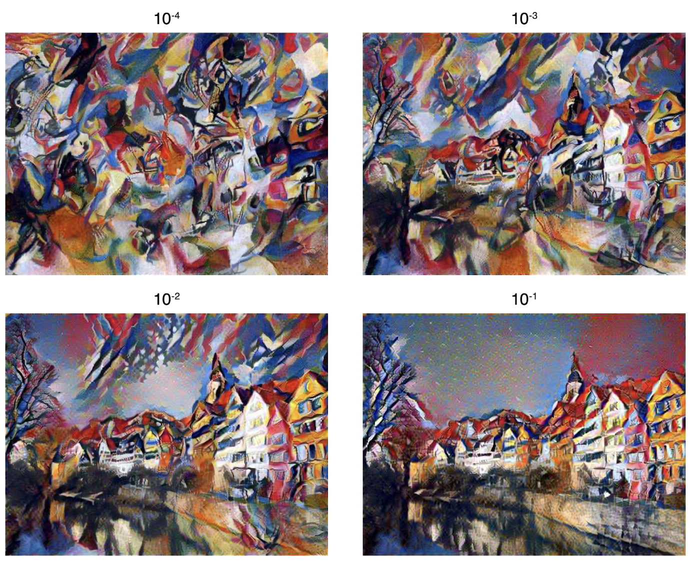
$\mathbf{Fig\ 8.}$ Relative weighting of matching content and style of the respective source images

Summary

In short, we summarize the pipeline of style transfer as following figure:

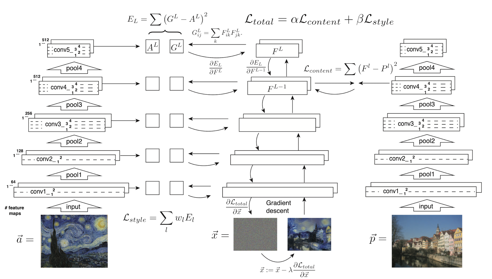
$\mathbf{Fig\ 9.}$ Style transfer algorithm

$\mathbf{Fig\ 10}$ shows a neural style transfer example that transfer the style of a photograph of New York by night onto an image of London in daytime:

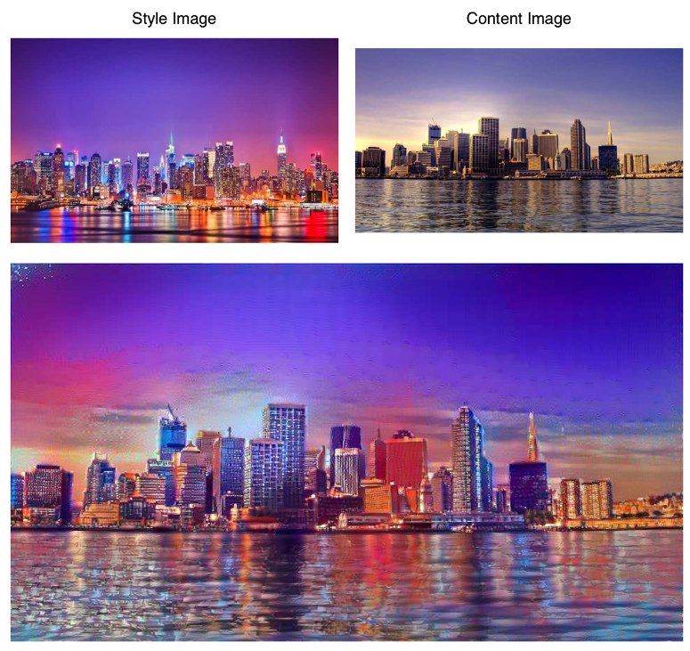
$\mathbf{Fig\ 10.}$ Relative weighting of matching content and style of the respective source images

Reference

[1] Gatys, Leon A., Alexander S. Ecker, and Matthias Bethge. “A neural algorithm of artistic style.” arXiv preprint arXiv:1508.06576 (2015).
[2] Gatys, Leon A., Alexander S. Ecker, and Matthias Bethge. “Image style transfer using convolutional neural networks.” Proceedings of the IEEE conference on computer vision and pattern recognition. 2016.
[3] UC Berkeley CS182: Deep Learning, Lecture 9 by Sergey Levine
[4] Wikipedia, Neural style transfer
[5] TensorFlow tutorial, Neural style transfer
[6] Lerner Zhang, Why we need the Gram matrix in style transfer learning?, URL (version: 2019-10-03)
[7] Li, Yanghao, et al. “Demystifying neural style transfer.” arXiv preprint arXiv:1701.01036 (2017).
[8] Gatys, Leon, Alexander S. Ecker, and Matthias Bethge. “Texture synthesis using convolutional neural networks.” Advances in neural information processing systems 28 (2015).