[CV] 3D Photography

Introduction

3D photography is a form of photography that captures perspectives of the world through a camera. It creates 3D viewing experiences through interactive adjustments of camera angles, using image-based rendering for novel view synthesis and delivers a dramatically more immersive experience compared to traditional 2D photography.

Neat introduction of 3D photography

In this post, we are interested in a problem that converting RGB-D image into 3D photo. An RGB-D image is a type of image that combines both color information and depth information. The depth information provides the distance of each pixel in the scene from the camera, creating a 3D representation of the environment. The depth can either come from dual camera cell phone stereo, or be estimated from a single RGB image.

Traditional image-based reconstruction and rendering methods demand intricate and specialized setups, often entailing dedicated hardware. However, contemporary approaches, exemplified by the Facebook 3D photo, now necessitate only a single snapshot captured with a dual-lens camera phone, essentially providing an RGB-D input image. Despite this convenience, these methods have their constraints; for instance, Facebook 3D photo employs an isotropic diffusion algorithm, yielding excessively smooth outcomes and struggling to extrapolate intricate textures and structures. This limitation has triggered the adoption of deep learning-based approaches for 3D photography tasks.

Modular-based v.s. Model-based

3D photography usually fall into 2 categories; modular-based approach and model-based approach (based on the end-to-end network).

• model-based approaches
  • aim to synthesize novel views on multi-view image datasets
  • typically take a single image as input and represent the scene using various representations (e.g. mesh, point cloud, multi-plane images) in an end-to-end manner
  • heavily depends on the training data and therefore cannot generalize to in-the-wild datasets.
• modular-based approaches
  • leverage the off-the-shelf state-of-the-art models for depth estimation, segmentation, or inpainting to produce reliable 3D experiences regardless the input data domain.
  • concentrate more on synthesis quality and computation efficiency.

In this regime, many recent works are built on modular-based approach rather than model-based.

3D Photo Inpainting (CVPR 2020)

The Layered depth image (LDI) representation is a view of the scene from a single input camera view, incorporating multiple pixels along each line of sight. Unlike a conventional 2D array of depth pixels (an RGB pixel with associated depth information D), it utilizes a 2D array of layered depth pixels. These layered depth pixels store a sequence of depth pixels along one line of sight, arranged in front-to-back order. The foremost element in the layered depth pixel samples the first surface encountered along that line of sight, with subsequent pixels in the sequence sampling the subsequent surfaces encountered along that line of sight, and so forth.

The following figure shows the example of LDI representation. LDIs are a useful representation for 3D photography, because

1. LDIs naturally handle an arbitrary number of layers, i.e., can adapt to depth-complex situations as necessary.
2. they are compact and sparse, i.e., memory and storage efficient and the size of the representation grows only linearly with the observed depth complexity in the scene. (As one can see, the number of valid pixels rapidly decreases as the index of the layer increases.)

$\mathbf{Fig\ 1.}$ Example of LDI representation (Liang Shi et al. 2022)

3D Photo Inpainting, proposed by Shih et al. 2020, takes as input an RGB-D image, converts RGB-D into LDI representation and generates a LDI with inpainted color and depth in parts that were occluded in the input. Although 3D Photo Inpainting requires trivial (i.e. one-layered) LDI, we can construct LDI with the arbitrary number of layers, using clustering algorithms. As an example, 3D Moments, CVPR 2022 first apply agglomerative clustering to separate the RGBD image into LDI with multiple layers , then perform context-aware color and depth inpainting for each layer.

$\mathbf{Fig\ 2.}$ RGB-D to inpainted LDI (Wang et al. CVPR 2022)

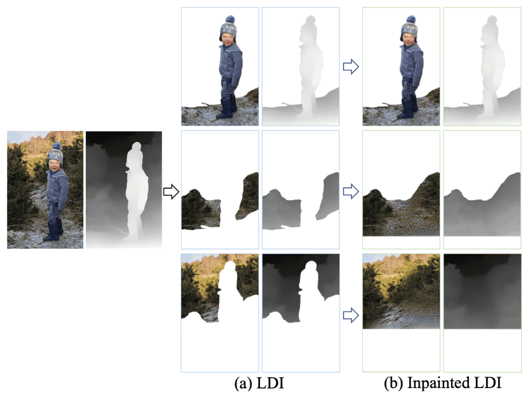
Image preprocessing

Context-aware layered depth inpainting firstly converts a RGB-D image into LDI representation. But instead of original LDI, it explicitly represents the local connectivity of pixels, by storing pointers in each pixel that points to either zero (at depth discontinuities) or at most one direct neighbor in each of the four directions ($\leftarrow$, $\rightarrow$, $\uparrow$, $\downarrow$).

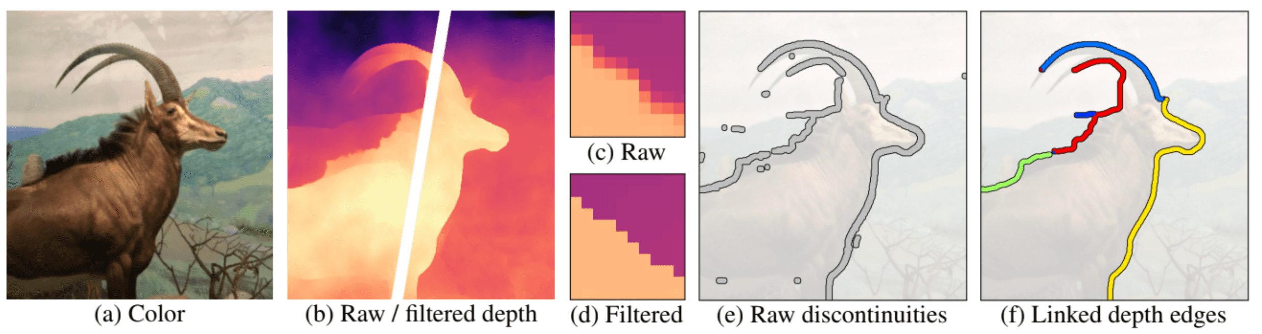
To inpaint the occluded parts of the scene, it identifies depth discontinuities. These are represented as blurred in most depth maps generated by stereo methods (such as dual camera cell phones) or depth estimation networks. However, the blur can make it challenging to precisely pinpoint the location of discontinuities. To address this, the depth maps are sharpened using a bilateral median filter.

$\mathbf{Fig\ 3.}$ Sharpening depth discontinuity (Shih et al. 2020)

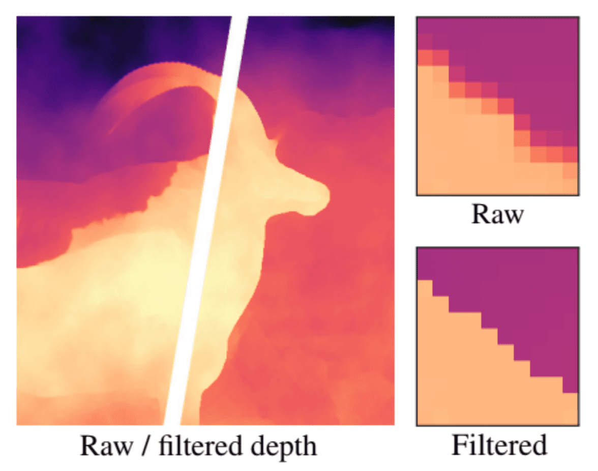
After sharpening the depth map, we identify discontinuities by thresholding the disparity difference between neighboring pixels. This results in many false positives, such as isolated speckles and short segments dangling off longer edges. To address this, the following steps are taken:

$\mathbf{Fig\ 4.}$ The results of each step of preprocessing (source: Shih et al. 2020)

1. Create a binary map, designating depth discontinuities as 1 and others as 0.
2. Conduct connected-component labeling to merge adjacent discontinuities into a set of linked depth edges. To address the edges at junctions, it is separated based on the local connectivity of the LDI.
   

   

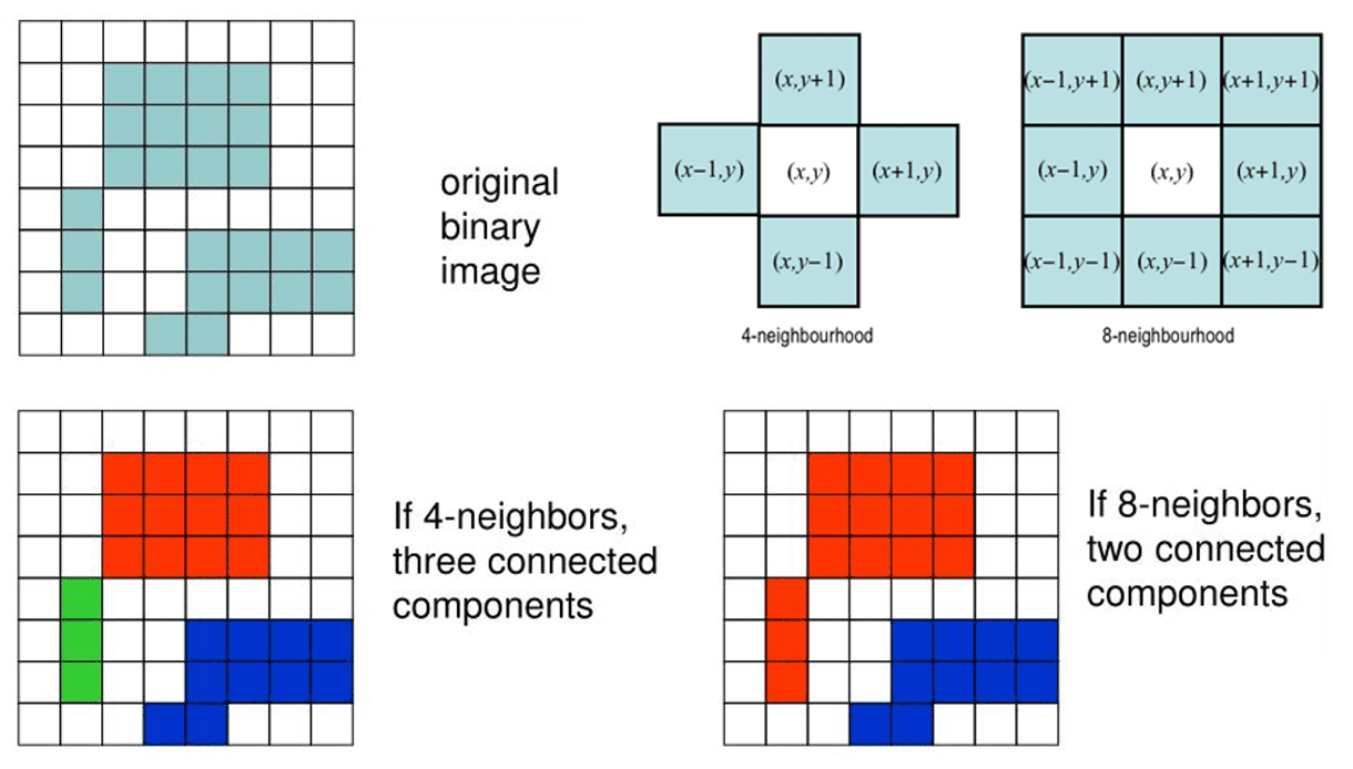
   $\mathbf{Fig\ 5.}$ Connected-component labeling

3. Remove short segments that the number of pixels is less than threshold, including both isolated and dangling ones. Empirically, the authors set threshold 10 pixels. The resulting edges form the basic unit of its iterative inpainting procedure, which is described in later.

Context and Synthesis regions

For inpainting problem formulation, the algorithm defines the context regions that aid inpainting of occluded parts, and synthesis regions that are required to be inpainted. These regions are formed from the depth edges (discontinuities) as follows.

$\mathbf{Fig\ 6.}$ LDI inpainting algorithm, illustrating foreground silhouette, background silhouette,
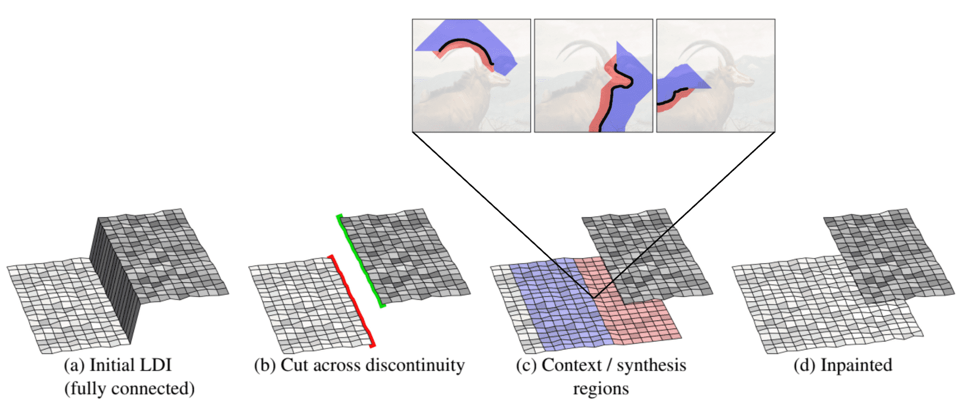
context region and synthesis region (source: Shih et al. 2020)

1. The LDI pixels are disconnected across the discontinuity and term silhouette pixels. Then the foreground silhouette and background silhouette (that equires inpainting) will form.
2. Create a synthesis region of 2D pixel coordinates (depth will be inpainted later) using a flood-fill algorithm. Starting from all silhouette pixels, the algorithm takes one step in the direction where they are disconnected. These pixels constitute the initial synthesis region. Subsequently, the region is iteratively expanded for 40 iterations by moving left/right/up/down and including any unvisited pixels. Notably, the algorithm avoids stepping back across the silhouette, ensuring that the synthesis region strictly remains in the occluded part of the image.

   

   $\mathbf{Fig\ 7.}$ Flood-fill algorithm (source: Wikipedia)

3. Similarly, create a context region of LDI pixel coordinates using a flood-fill algorithm for 100 iterations, but following their connection links of LDI pixels. The inpainting networks only considers the content in the context region and does not see any other parts of the LDI.
4. In practice, the silhouette pixels may not align well with the actual occluding boundaries due to imperfect depth estimation. To tackle this issue, we dilate the synthesis region near the depth edge by 5 pixels (the context region erodes correspondingly).

   

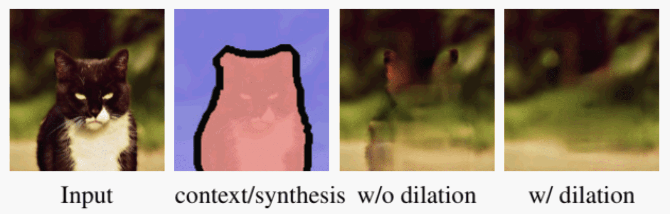
   $\mathbf{Fig\ 8.}$ Handling imperfect depth edges (source: Shih et al. 2020)
   
   

Context-aware color and depth inpainting

The inpainting task is divided into 3 sub-problems:

1. Edge inpainting network
   • Inpaint the edges in the synthesis region based on the context region
   • It helps infer the structure (in terms of depth edges) that can be used for constraining the content prediction
2. Color inpainting network
   • Input: concatenated inpainted edges and context color
   • Output: inpainted color
3. Depth inpainting network
   • Input: concatenated inpainted edges and context depth
   • Output: inpainted depth

$\mathbf{Fig\ 9.}$ The framework of the inpainting algorithm (source: Shih et al. 2020)

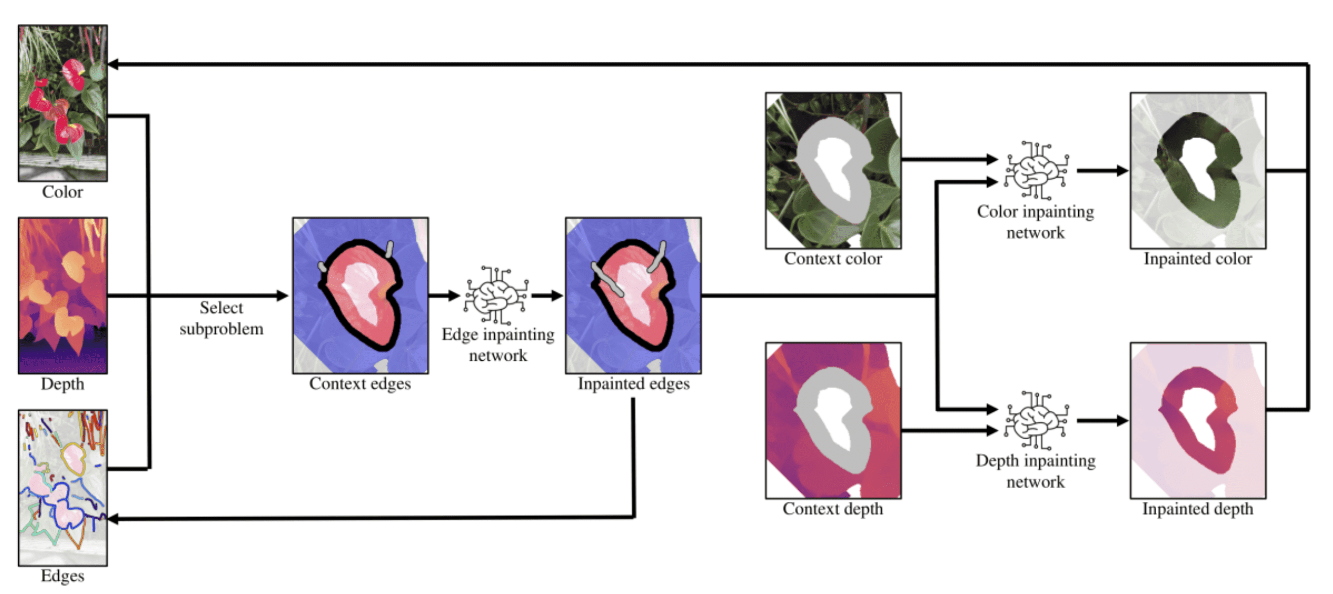
The edge-guided inpainting extends the depth structures accurately and mitigates the color/depth misalignment issue.

$\mathbf{Fig\ 10.}$ Effect of edge-guided inpainting (source: Shih et al. 2020)

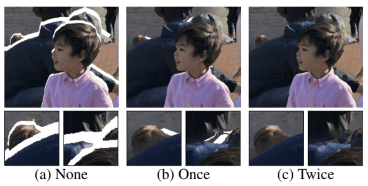
Furthermore, in situations with depth complexity, a single application of the inpainting model may not be adequate, as the hole might still be visible through the discontinuity created by the inpainted depth edges. Therefore, the algorithm iteratively applies the inpainting process until no further inpainted depth edges are generated.

$\mathbf{Fig\ 11.}$ Multi-layer inpainting (source: Shih et al. 2020)

Result

$\mathbf{Fig\ 12.}$ Visual comparison to Facebook 3D Photos (source: Shih et al. 2020)

Diffuse3D (ICCV 2023)

3D Photo Inpainting relies on modular systems and leverage state-of-the-art depth estimation, inpainting, and segmentation models to understand the LDI representation and fill in the holes of occlusions. This component-wise approach exhibits robust performance in handling diverse real-world scenes. However, due to the limited and narrow boundary context for inpainting, it is constrained to small camera view angle changes (generally 5-10 consecutive frames for one scene), limiting the creation of a truly immersive experience.

Extending the camera angle reveals larger occluded regions that cannot be simply filled by duplicating neighboring textures. But human could conjecture the occluded areas not only from the nearby visible areas but also by connecting to the visual memories. Hence, inspired by this heuristic, Diffuse3D from Y Jiang et al. ICCV 2023 employs an pre-trained latent diffusion model as the generative prior, and further empowers it to be depth-aware by introducing bilateral convolution into the denoising inference process.

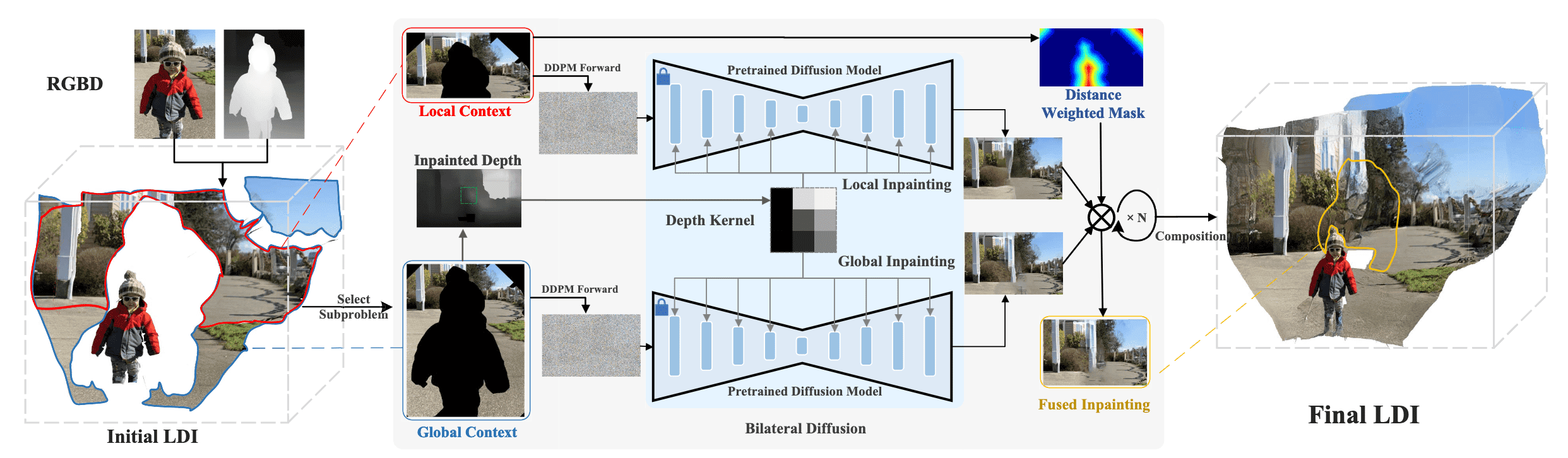
The following figure shows the overall pipeline of Diffuse3D. Firstly, it selects one edge from the depth edges and expands the synthesized regions and context regions along the edge by the flood-fill algorithm, similar to 3D Photo Inpainting. Then, a depth inpainting network is employed to synthesize depth $D$ in the occluded regions. Unlike 3D Photo Inpainting, which carries out color inpainting independently from depth, Diffuse3D leverages depth to encourage color inpainting results with color-depth consistency.

$\mathbf{Fig\ 13.}$ Diffuse3D framework (Y Jiang et al. 2023)

Bilateral Diffusion

The denoising network in the usual latent diffusion model is UNet-based convolutional network. Hence for the $\ell$-th layer in the denoising network, a specific pixel at the spatial coordinate $p$ is computed through the denoising process as follows:

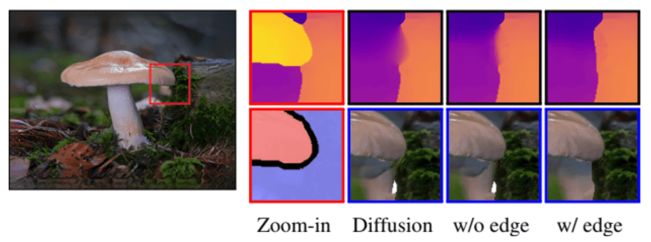
\[\begin{aligned} y(p) = \sum_{p_i \in \Omega} x(p_i) g_s (\lVert p_i - p \rVert) \end{aligned}\]

where $\Omega$ is the window centered at $p$ and $g_s$ is the spatial kernel of denoising model. But the standard CNNs are limited to model geometric transformations due to the fixed structure of convolution kernels. It exhibits translation invariance and treats pixels of different depths equally, leading to synthesis content with color-depth inconsistency near the depth edges.

$\mathbf{Fig\ 14.}$ A and C are labeled as a table, while B is designated as a chair, sharing similar visual features in the RGB image but distinguished in depth. Depth-aware CNNs consider geometric relations in both convolution and pooling. When A is the receptive field center, C contributes more to the output than B. (W Wang et al. 2018)

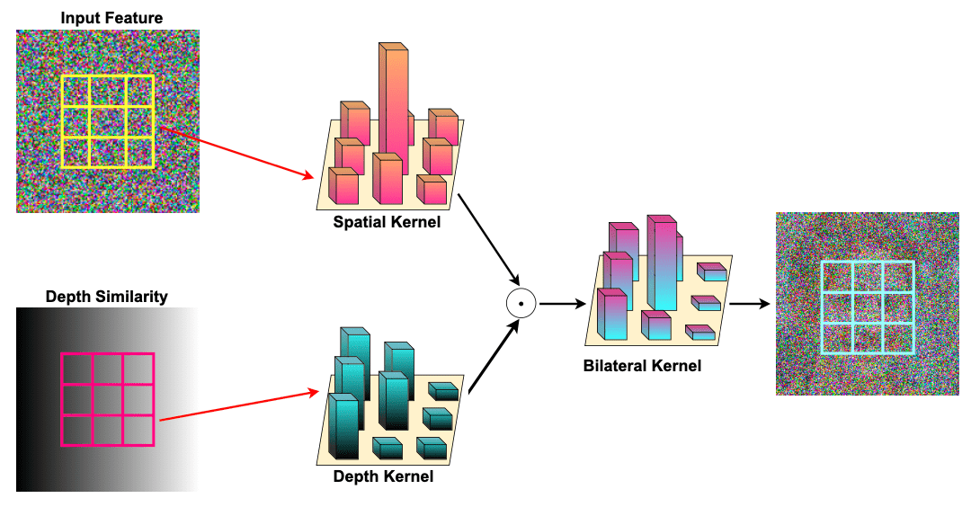
The authors proposed bilateral diffusion, which leverage depth information for inpainting to preserve color-depth consistency. The convolutional kernel in bilateral diffusion consists of two types of kernel:

• spatial kernel $g_s$: standard convolution filter
• depth kernel $f_d$: weight filter computed by the depth differences with the center pixels.

\[\begin{aligned} f_d (\lVert D (p_i) - D(p) \rVert) = \exp \left( - \frac{\lVert D (p_i) - D(p) \rVert}{2\sigma_r^2} \right) \end{aligned}\]

The selection of $f_d$ is based on the intuition that pixels with similar depths should have more impact on each other. Then, we apply the depth kernel to reweight the spatial filter:

\[\begin{aligned} y(p) = \sum_{p_i \in \Omega} x(p_i) g_s (\lVert p_i - p \rVert) f_d (\lVert D (p_i) - D(p) \rVert). \end{aligned}\]

$\mathbf{Fig\ 15.}$ Bilateral convolution (Y Jiang et al. 2023)

In this way, depth prior is injected in the diffusion model and the bilateral diffusion concerns more on the pixels with similar depth. Note that the gradients for $\mathbf{x}$ and $g_s$ are simply multiplied by $f_d$. Note that the $f_d$ part doesn’t integrate any parameters to bilateral diffusion.

Cross-layer Inpainting

Intuitively, the foreground layers of depth edges might encompass irrelevant content, potentially leading to misguidance in the background inpainting process. Therefore, they should be excluded from the context regions. According to the intuition, the authors broaden the context regions from the layer close in depth to all background layers—those positioned beyond the current layer.

Moreover, to obtain diverse contextual knowledge, the authors divide the context into two branches.

• local context
  • the regions close (in depth) with synthesis regions
  • identified by flood-fill algorithm
  • equivalent to the context region in 3D Photo Inpainting
• global context: the other regions beyond the synthesis region in depth

$\mathbf{Fig\ 16.}$ Demonstration for synthesis and context regions (Y Jiang et al. 2023)

The authors apply the inpainting model to each branch independently, and for each pixel in occluded region, fuse the inpainted images into a composite image by a distance-based weighted fusion as below.

\[\begin{aligned} w = \frac{d_{\text{edge}}}{\max (d_{\text{edge}})}, \quad y = w \cdot y_{\text{local}} + (1-w) \cdot y_{\text{global}} \end{aligned}\]

where $w$ is the weight for the local-global fusion and $d_{\mathrm{edge}}$ denotes the distance between the occluded pixel and the depth edge. By considering global context more than local context in occluded pixels nearby depth discontinuity, it can alleviate the large change on depth of background, leading to natural and realistic inpainted results.

Result: On Challenging Scenarios

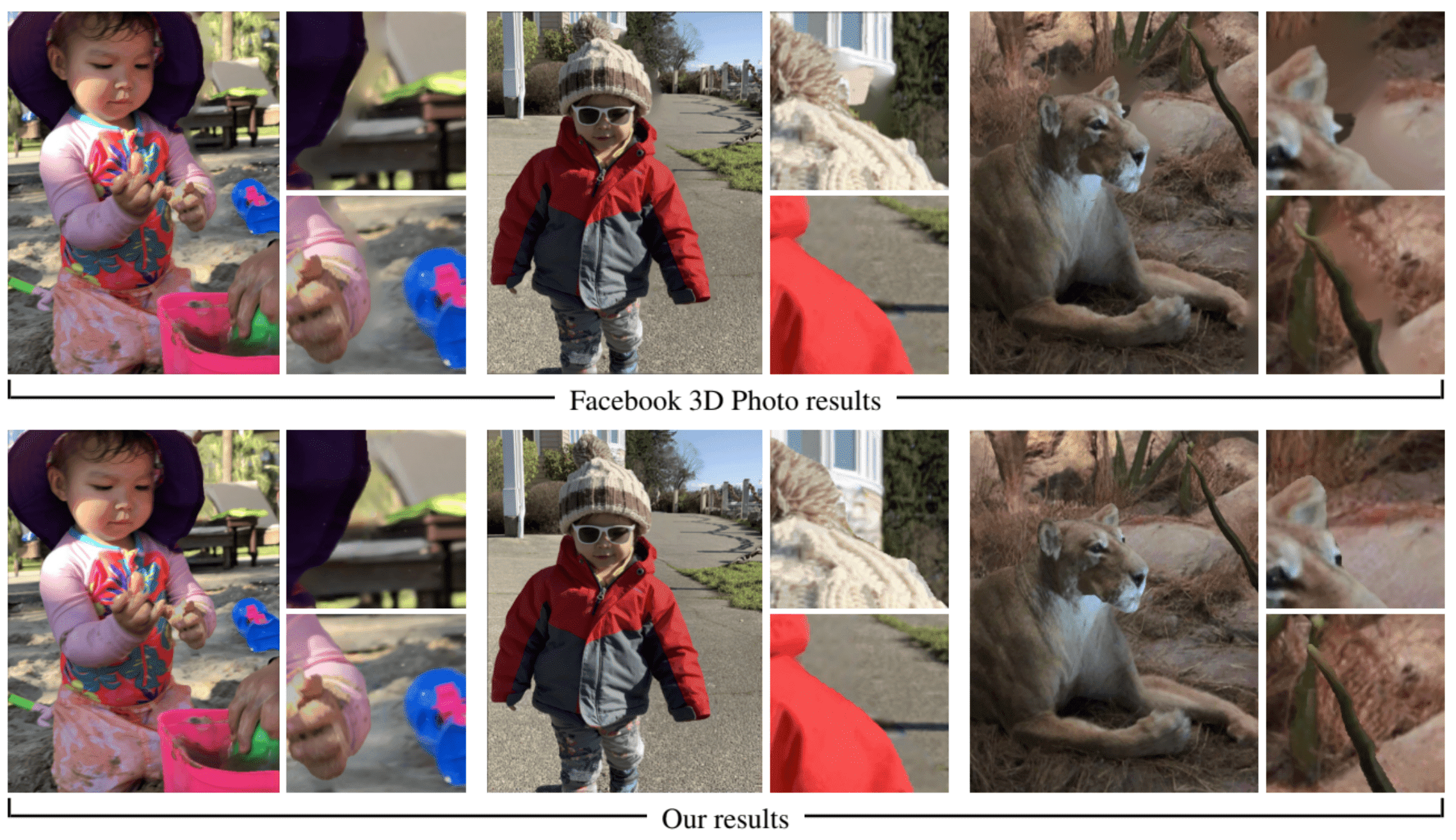
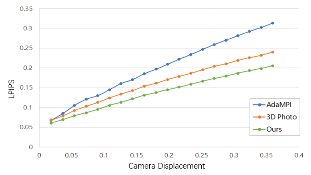
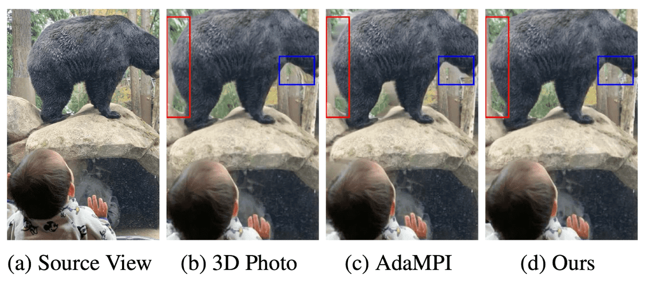
In handling wide-angle camera movements, Diffuse3D exhibits more promising results than 3D Photo. This suggests that bilateral diffusion efficiently directs the denoising model to prioritize pixels in close depth proximity, filtering out extraneous foreground details and thereby enhancing synthesis quality. Moreover, our introduced global-local inpainting strategy serves to further augment the overall quality of synthesis.

$\mathbf{Fig\ 17.}$ Comparison of wide-angle movement (Y Jiang et al. 2023)

And in handling scene with multiple foregrounds, the outcome illustrates that Diffuse3D understands geometric relationships adeptly, yielding more realistic results compared to alternative methods.

$\mathbf{Fig\ 18.}$ Scene with Multiple Foregrounds (Y Jiang et al. 2023)

Reference

[1] Shih et al., “3D Photography using Context-aware Layered Depth Inpainting”, CVPR 2020
[2] Jiang et al., “Diffuse3D: Wide-Angle 3D Photography via Bilateral Diffusion”, ICCV 2023
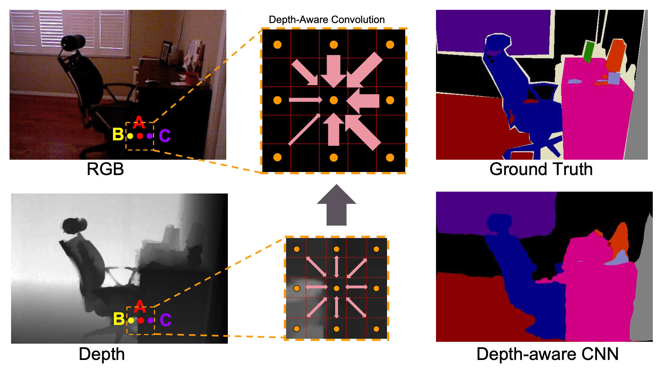
[3] Wang et al., “Depth-aware CNN for RGB-D Segmentation”, ECCV 2018
[4] Wang et al., “3D Moments from Near-Duplicate Photos”, CVPR 2022