
[CV] Camera View Adjustment
Introduction
Image composition has a crucial effect on the perception of an image and contributes to the quality of a photo. However, general users don’t possess the knowledge and expertise required to capture images with great composition. This arised huge interest for the assistance systems and aesthetic assessment method for photography. (e.g. shot suggestion function of Samsung Galaxy S10)
Camera View Adjustment Prediction
Approach
The pioneering work in deep learning-based view adjustment is the camera view adjustment prediction proposed by Su et al., 2021 from Google Research. Given a photo taken by the user, the proposed sysytem provides a suggested view adjustment and its magnitude represented by a percentage of the image size or radians. In contrast to the previous image adjustment methods that only consider the cropping, it supports more generic modifications:
- horizontal (left/right) move
- vertical (up/down) move
- zoom (in/out)
- rotation (clockwise/counter clockwise)
The main challenge of view adjustment is the absence of the dataset for evaluating the performance of view adjustment prediction. To address this issue, the paper generates the sample images and ground truth image from existing image cropping datasets by converting view adjustments into operations on 2D image bounding boxes and use the best crop annotation as the target view for adjustment.
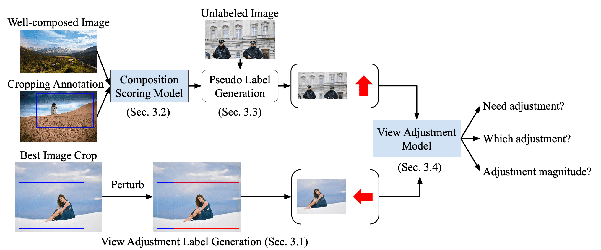
Since the system generates training samples from the image cropping datasets, the distribution and diversity of the generated data is heavily inherited from the source datasets. Although CNNs require a large and diverse dataset for training, the recent image cropping datasets usually come from a relatively small number of images. To increase the amount & diversity of training data and improve model performance, the system further leverages additional unlabeled images that are out of image cropping dataset. The training system operates in two-stages as follows:
- Composition Scoring Model
As the first stage, the MobileNet-based composition scoring model $M_c$ that takes an RGB image as input and outputs a score in $[0, 1]$. Let $(\mathbf{I}_p, \mathbf{I}_n)$ be two images of the same scene where $\mathbf{I}_p$ has the better composition. To guide the model to compare the results of different view adjustments, define the pairwise ranking loss that encourages the score of $\mathbf{I}_p$ to be more than that of $\mathbf{I}_n$ by a margin $\delta > 0$: $$ \max ( 0, \delta - [M_c (\mathbf{I}_p) - M_c (\mathbf{I}_n)]) $$ To train the composition scoring model, the image pairs $(\mathbf{I}_p, \mathbf{I}_n)$ are generated in 3 different ways.-
Labeled data
-
Scored candidate crops
Each image comes with a dataset of candidate crops along with their scores. In each training iteration, choose $N$ crops from a random image and generate $N(N −1)/2$ pairs. Afterwards, $\mathbf{I}_p$ and $\mathbf{I}_n$ are determined for each pair by comparing the provided scores. The computed pairwise ranking loss averaged over these $N(N−1)/2$ pairs is denoted as $\mathcal{L}_{\text{sc}}$. -
Best crop annotation
In this format, a best crop for each image is provided. Then, generate $K$ number of $\mathbf{I}_n$ by randomly perturbing (randomly shifting/zooming-out/cropping/rotation) the bounding box of the best crop $\mathbf{I}_p$. The computed pairwise ranking loss averaged over these $K$ pairs is denoted as $\mathcal{L}_{\text{bc}}$.
Note that supervised samples where the perturbed bounding box goes beyond the original image are discarded. -
Scored candidate crops
-
Unlabeled data
First, collect well-composed images $\mathbf{I}_p$ contributed by experienced photographers. Then, it randomly perturbs the image to generate $P$ number of new images with poor composition, denoted as $\mathbf{I}_n$. The computed pairwise ranking loss averaged over these $P$ pairs is denoted as $\mathcal{L}_{\text{wc}}$.
Unlike the perturbation in the labeled data, in unlabeled data, it is allowed to go beyond the original image. Unknown regions are filled with zero pixels.
Therefore, the total loss function used to train the composition scoring model is given by $\mathcal{L} = \mathcal{L}_{\text{sc}} + \mathcal{L}_{\text{bc}} + \mathcal{L}_{\text{wc}}$. The figure below outlines the training pseudocode.
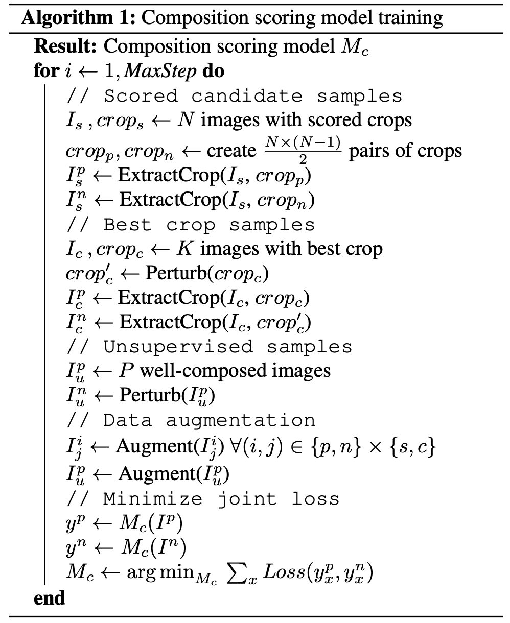
$\mathbf{Fig\ 2.}$ Composition scoring model training (Su et al. 2021)
-
Labeled data
- Pseudo Label Generation
Next, generate pseudo view adjustment labels using the composition scoring model through simulation. Given an image, generate the results of 8 view adjustments with 9 different magnitudes for each operation, equally spaced between:- $[\pi/36, \pi/4]$ for rotation
- $[5\%, 45\%]$ for other modifications
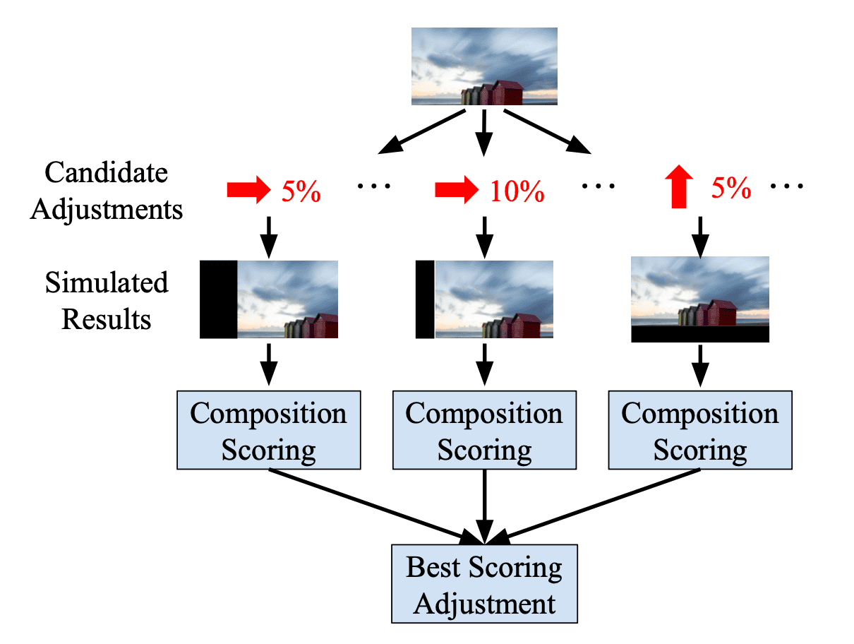
$\mathbf{Fig\ 3.}$ Pseudo-Label Generation (Su et al. 2021)
- View Adjustment Model
Given the labeled samples from the view adjustment dataset and the images with pseudo label generated by the composition scoring model, the MobileNet-based view adjustment model with 3 output heads is trained:-
Suggestion predictor
A binary classification head that outputs whether a view adjustment should be suggested, trained with cross-entropy loss -
Adjustment predictor
A multi-class classification head that outputs the index for required adjustment, trained with categorical cross-entropy loss -
Magnitude predictor
8 regressors that regress the adjustment magnitude for each of the candidate adjustments, trained with $L_1$ loss
The figure below outlines the training pseudocode.
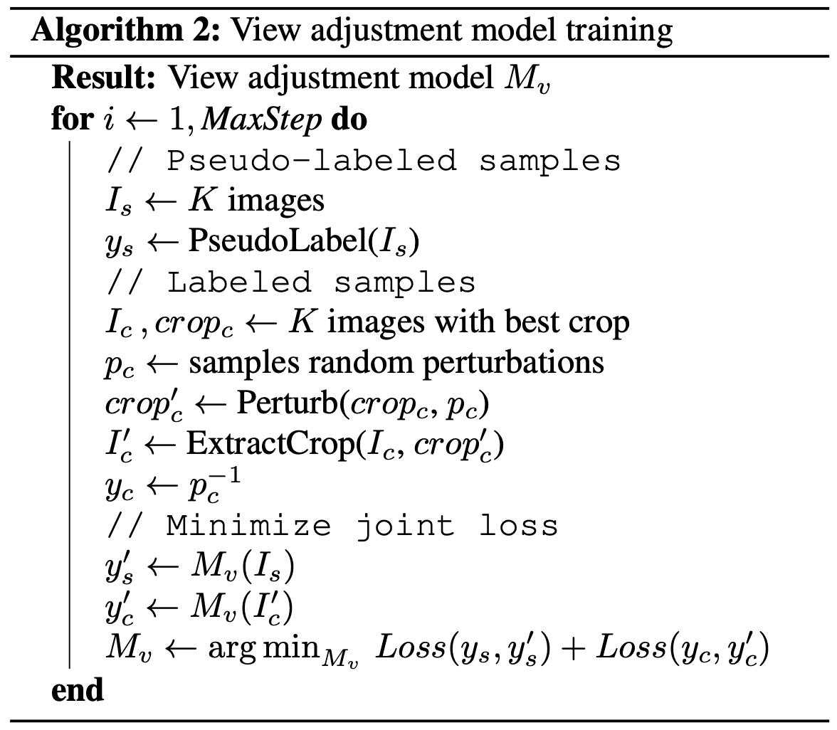
$\mathbf{Fig\ 4.}$ View adjustment model training (Su et al. 2021)
-
Suggestion predictor
Result
To demonstrate the effectiveness of the proposed two-stage semi-supervised training approach, they compared the following variants of the proposed methods:
- Supervised – The view adjustment model is trained using only the labeled data, and the unlabeled images are not used.
- Aesthetic-scoring – It uses aesthetic scores to train the image scoring model; the scoring model is trained to regresses the mean opinion scores of 250K images from the AVA dataset, a widely-used image aesthetics dataset.
- Supervised-scoring – The composition scoring model is trained using only labeled data, and the unlabeled images are not used.
And the following table shows the excellency of proposed strategy against other variants, except for the Zoom-in and Counter clockwise rotation adjustment. It can be elucidated by the distribution of adjustment magnitudes, where most of zoom-in and rotation samples exhibit subtle perturbation magnitudes due to unknown regions, rendering them intrinsically more challenging for accurate view adjustment prediction.
The results further imply the significance of semi-supervised learning to not only for the view adjustment model but also for the composition scoring model. To train the composition scoring model using only supervised data yields worse results than the purely supervised view adjustment model. It is potentially attributed to the poor quality of pseudo labels generated by the supervised composition scoring model, which is trained on a limited number of images. Moreover, the performance of Aesthetic-scoring is much inferior than others, underscoring that a generic aesthetic score is insufficient to differentiate the changes of composition.

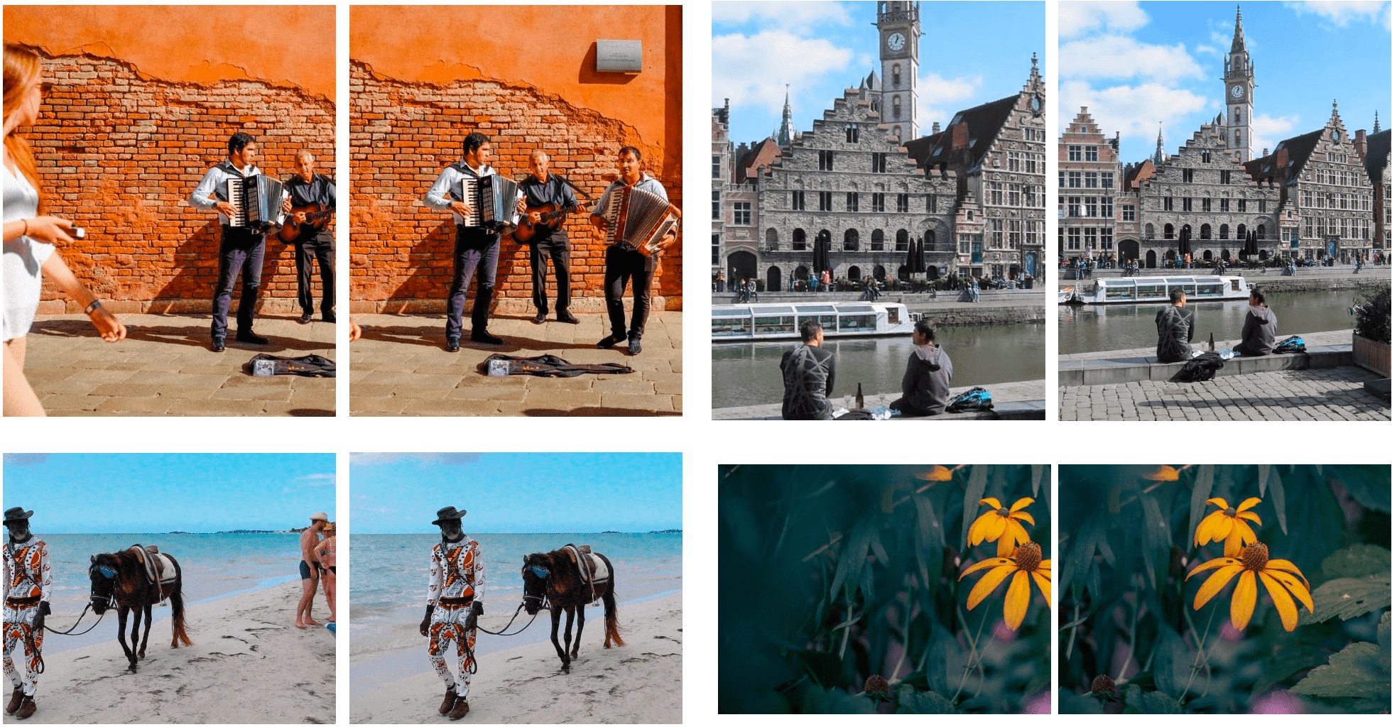
Since there is no prior published work on view adjustment models and evaluation metrics for image composition, it is hard to measure the effectiveness of the system by conducting quantitative analysis. Instead, the qualitative results suggest that the model provide suggestions based on various factors, including objects, the ground plane, or even leading lines in the image. $\mathbf{Fig\ 5.}$ shows some qualitative examples.
However, the model fails in some cases, for example when the target adjustment is minor or the important content is not visible in the initial view, exhibiting the following failure examples.
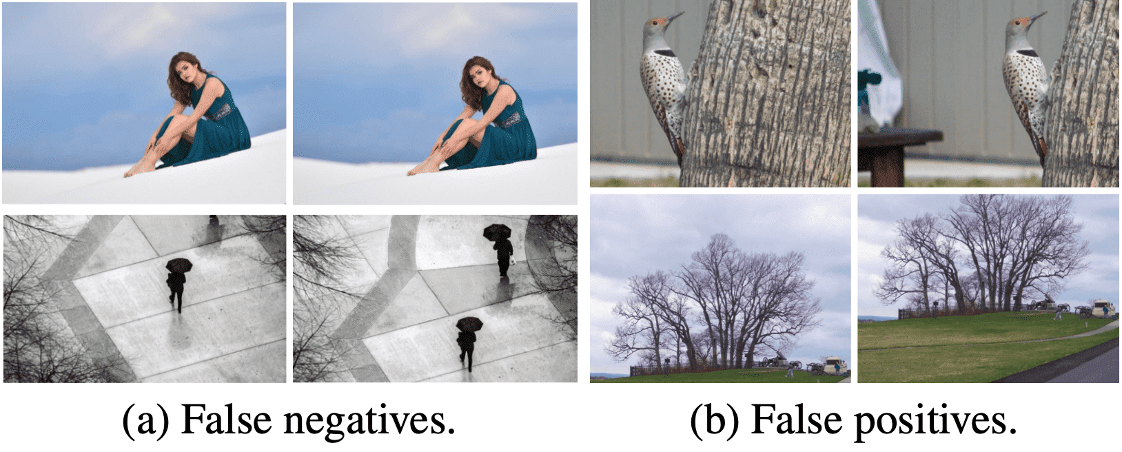
FN: the model fails to provide a suggestion when the composition can be improved.
FP: the suggested adjustment degrades the composition according to the user study.
Image Composition Assessment
The composition scoring model is the key factor of camera view adjustment prediction system discussed in the previous section, and plays a part as the expert that provides the supervision during training and suggests the adjustment in inference session. Unfortunately, Due to the lack of the prior works and datasets on image composition rating, the authors manually trained the network without any explicit consideration of composition ingredients such as visual balance, composition rules (e.g., rule of thirds, diagonals and triangles), etc. However in the same year, Zhang et al. BMVC 2021 firstly constructs the composition assessment dataset and proposes the image composition assessment networks trained on that dataset called SAMP-Net.
Composition Assessment DataBase (CADB)
Despite the importance of image composition, there was no dataset readily available for image composition assessment until recently. Some existing aesthetic datasets contain annotations related to image composition, but they only have composition-relevant attributes without overall composition score or are rated by unprofessionals.
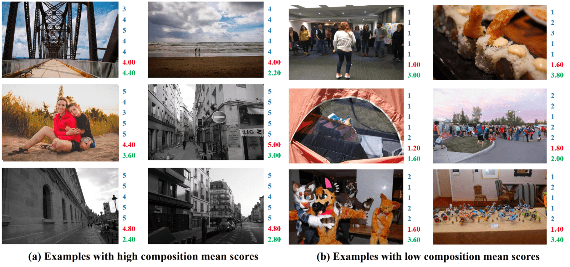
On the basis of Aesthetics and Attributes DataBase (AADB) dataset, the first image composition assessment dataset called Composition Assessment DataBase (CADB) is proposed by Zhang et al. BMVC 2021. It contains 9,497 images with each image rated from 1 to 5 by five individual raters who specialize in fine art for the overall composition quality.
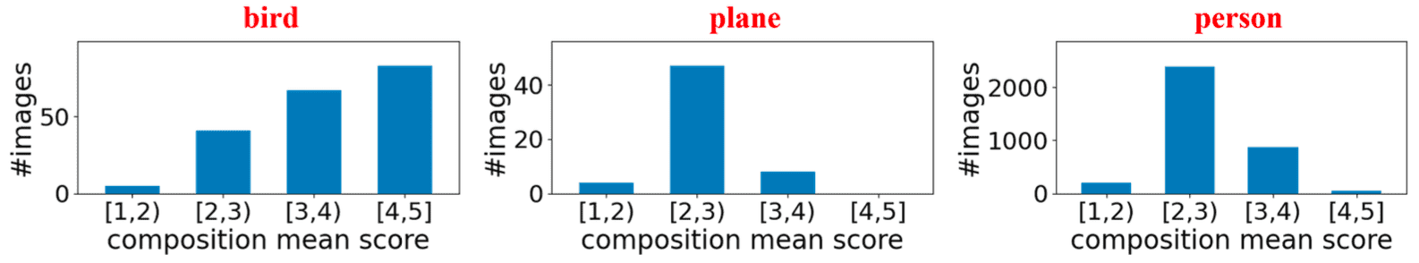
However, it is imperative to note that some content bias exist in the dataset; certain categories of photos exhibit the score distributions concentrated within very narrow intervals. For example, most bird photos are rated with high scores, probably because they are more likely to be taken by professional photographers rather than amateurs. In such scenarios, the network might inadvertently exploit this bias to simply rate images rather than nuanced compositional elements.
SAMP-Net
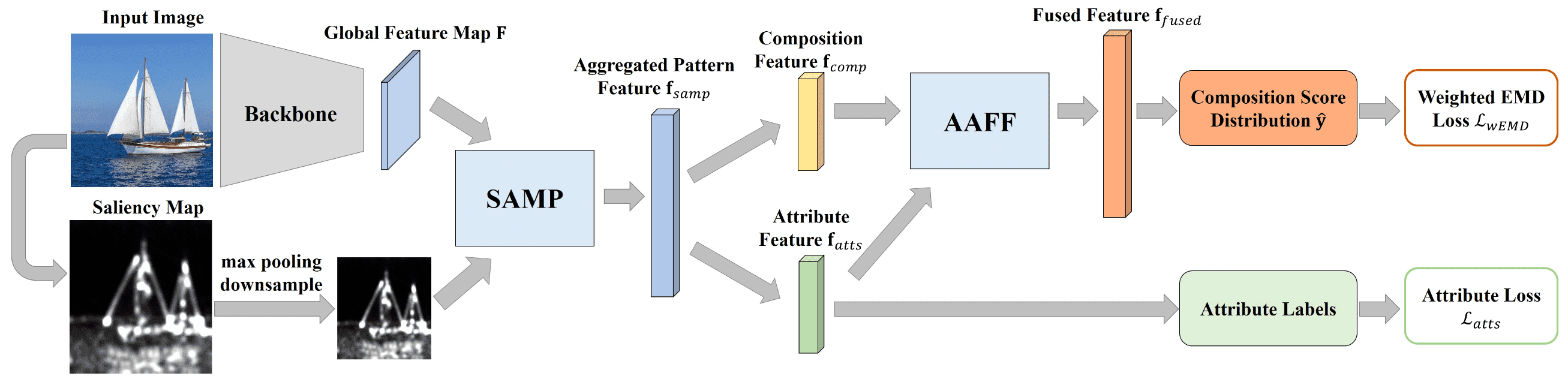
Training on CADB, Zhang et al. 2021 propose a composition assessment network termed SAMP-Net with a novel Saliency-Augmented Multi-pattern Pooling (SAMP) module, which analyses visual layout from the perspectives of multiple composition patterns.
Saliency-augmented Multi-pattern Pooling
Composition pattern is an important respect of composition assessment. By analyzing the visual layout according to composition pattern, for example comparing the visual elements in various partitions, we can quantify the aesthetics of visual elements in terms of visual balance, composition rules (e.g., rule of thirds, diagonals and triangles), and others. Thus, different composition patterns can also provide different perspectives to evaluate composition quality.
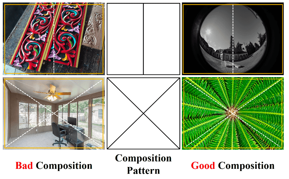
Inspired from this observation, Zhang et al. 2021 propose a multi-pattern pooling at the end of feature extractor backbone to integrate the visual information extracted from multiple patterns. Considering that the sizes and locations of salient objects are representative of visual layout and fundamental to image composition, we further incorporate the saliency information (i.e., locations and scales of salient objects) into multi-pattern pooling, leading to Saliency-augmented Multi-pattern Pooling (SAMP) module:
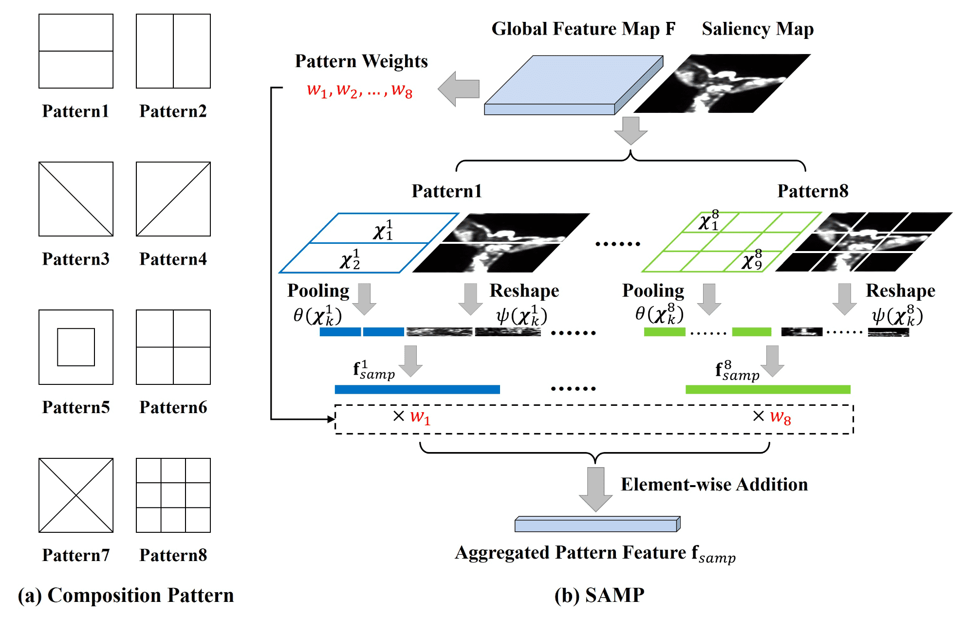
Given a global feature map $\mathbf{F} \in \mathbb{R}^{H \times W \times C}$ extracted from input image by backbone, denote the pixel-wise feature at each location as \(\mathbf{F}_{i,j} \in \mathbb{R}^{C}\) ($1 \leq i \leq H$, $1 \leq j \leq W$). For the $p$-th composition pattern, divide $\mathbf{F}$ into $K_p$ non-overlapping partitions \(\{\mathcal{X}_1^p, \mathcal{X}_2^p, \cdots, \mathcal{X}_{K_p}^p \}\) through its composition. And for each partition element, apply average pooling to obtain the partition feature:
\[\theta(\mathcal{X}_k^p) = \frac{1}{\lvert \mathcal{X}_k^p \rvert} \sum_{(i, j) \in \mathcal{X}_k^p} \mathbf{F}_{i, j} \in \mathbb{R}^C\]Next, produce saliency maps $\mathbf{S} \in \mathbb{R}^{H_{\text{sal}} \times W_{\text{sal}} = 8H \times 8W}$ for input image via unsupervised saliency detection method. Note that the size of saliency map is much larger than global feature map, so as to retain more details of salient objects. Then again, obtain $K_p$ non-overlapping partitions \(\{\mathcal{X}_1^p, \mathcal{X}_2^p, \cdots, \mathcal{X}_{K_p}^p \}\) for $p$-th pattern. Instead of average pooling that leads to the loss of information, compute the partition feature $\psi (\mathcal{X}_k^p) \in \mathbb{R}^{D_k^p}$ by simply reshaping $\mathbf{S}$. Finally, obtain the pattern vector by applying FC layer to the concatenated partition feature $[\psi (\mathcal{X}_k^p), \theta(\mathcal{X}_k^p)]$:
\[\mathbf{f}_{\text{samp}}^p = \operatorname{ReLU}(\operatorname{FC}([\psi (\mathcal{X}_1^p), \theta(\mathcal{X}_1^p), \cdots, \psi (\mathcal{X}_{K_p}^p), \theta(\mathcal{X}_{K_p}^p)]))\]Since some composition patterns may play more important roles when evaluating image composition, our model is trained to assign different weights for different patterns to fuse multi-pattern features:
\[\mathbf{f}_{\text{samp}} = \sum_{p=1}^P w_p \cdot \mathbf{f}_{\text{samp}}^p\]where $P$ is the number of composition patterns and $w_p$ is learnable weight.
Attentional Attribute Feature Fusion
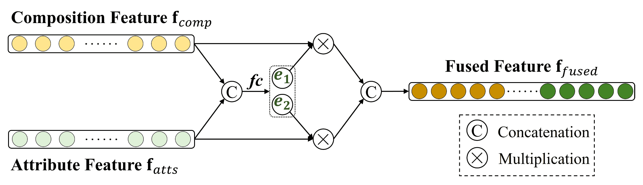
To help composition assessment, SAMP-Net further leverages composition-relevant attributes (rule of thirds, balancing elements, object emphasis, symmetry, and repetition). In specific, decompose the aggregated pattern feature \(\mathbf{f}_{\text{samp}} \in \mathbb{R}^{C^\prime}\) into composition feature \(\mathbf{f}_{\text{comp}} \in \mathbb{R}^{C^\prime/2}\) and attribute feature \(\mathbf{f}_{\text{atts}} \in \mathbb{R}^{C^\prime/2}\) via two individual fc layers:
\[\begin{aligned} \mathbf{f}_{\text{comp}} & = \operatorname{FC}_1 (\mathbf{f}_{\text{samp}}) \\ \mathbf{f}_{\text{atts}} & = \operatorname{FC}_2 (\mathbf{f}_{\text{samp}}) \\ \end{aligned}\]And dynamically weigh the contributions of two features and produce the fused feature \(\mathbf{f}_{\text{fused}}\):
\[\mathbf{f}_{\text{fused}} = [e_1 \mathbf{f}_{\text{comp}}, e_2 \mathbf{f}_{\text{atts}}] \in \mathbb{R}^{C^\prime} \text{ where } [e_1, e_2] = \operatorname{sigmoid}(\operatorname{FC}([\mathbf{f}_{\text{comp}}, \mathbf{f}_{\text{atts}}]))\]
Training Loss
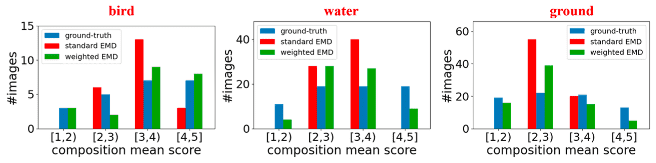
During training, an additional layer is attached to perform attribute prediction based on the attribute feature \(\mathbf{f}_{\text{atts}}\) with MSE loss \(\mathcal{L}_{\text{atts}}\). Furthermore, to mitigate the content bias in training set, SAMP-Net is also trained to minimize weighted EMD loss \(\mathcal{L}_{\text{wEMD}}\) which assigns smaller weights to biased samples when calculating EMD Loss. To calculate the loss, first identify the biased categories using Faster R-CNN object detector and divide the range of composition mean score $\bar{y}$ into $M = 4$ bins with the equal size of $1$. Then, the category with an entropy below $1.5$ is treated as a biased category. Then, the weighted EMD loss can be computed by
\[\mathcal{L}_{\text{wEMD}} (\mathbf{y}, \hat{\mathbf{y}}) = \left( \frac{1}{S} \sum_{s=1}^S \beta \times \lvert \operatorname{CDF}_{\mathbf{y}} (s) - \operatorname{CDF}_{\hat{\mathbf{y}}} (s) \rvert^r \right)^{1/r}\]where $S = 5$ is the scale of composition score in the dataset, $r$ is a hyper-parameter, and \(\operatorname{CDF}_{\mathbf{y}} (s) = \sum_{i=1}^s y_i\) denotes the cumulative distribution function. The weight $\beta$ for given an image that contains $C$ object categories and has the composition mean score $\bar{y}$ falling in the $m$-th bin, can be computed by
\[\beta = \min \{ \alpha_{m, 1}, \alpha_{m, 2}, \cdots, \alpha_{m, C} \}\]where $\alpha_{m, c} = \sum_{i=1}^M T_{i, c} / ( M \cdot T_{m, c} )$ and $T_{m, c}$ is the occurrence that the $c$-th category appears in $m$-th bins.
Finally, SAMP-Net is optimized in an end-to-end manner with these losses: \(\mathcal{L} = \mathcal{L}_{\text{wEMD}} + \lambda \mathcal{L}_{\text{atts}}\) where $\lambda$ is a trade-off parameter set as $\lambda = 0.1$ via cross validation.
Result
As a result, the SAMP-Net clearly outperforms all the composition-relevant baselines, which demonstrates that it is more adept at image composition assessment.
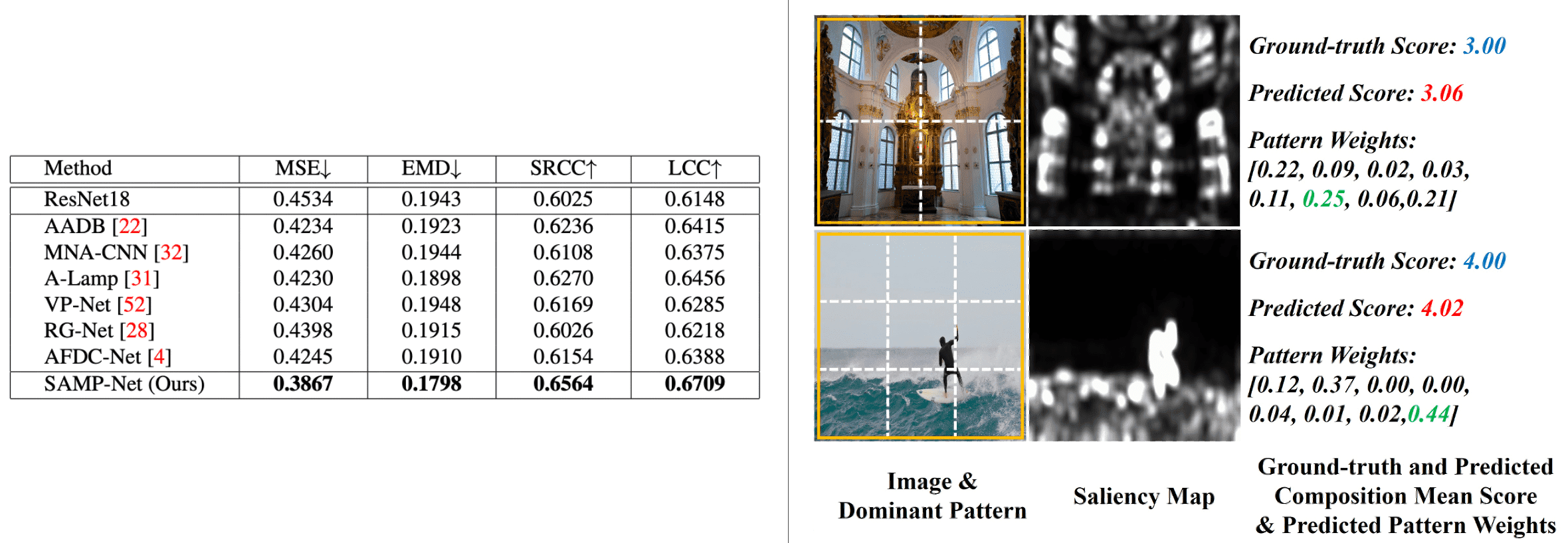
(Right) Analysis of the correlation between an image and its dominant pattern with the largest weight.
(Zhang et al. 2021)
Reference
[1] Su et al., “Camera View Adjustment Prediction for Improving Image Composition”, arXiv preprint arXiv:2104.07608 (2021).
[2] Zhang et al., “Image Composition Assessment with Saliency-augmented Multi-pattern Pooling”, BMVC 2021.
Leave a comment