
[CV] Resolution-Free ViT
In the field of computer vision, the limitation of vision models to fixed resolutions has been a long-standing challenge, which is originated from the efficient processing on contemporary hardware. Deep neural networks are typically trained and run with batches of inputs, thus necessitating fixed batch shapes and fixed image sizes. And this constraint often leads to the ubiquitous and demonstrably suboptimal choice of resizing or padding images before processing them. Both of these have been shown to be flawed: the former harms performance and the latter is inefficient.
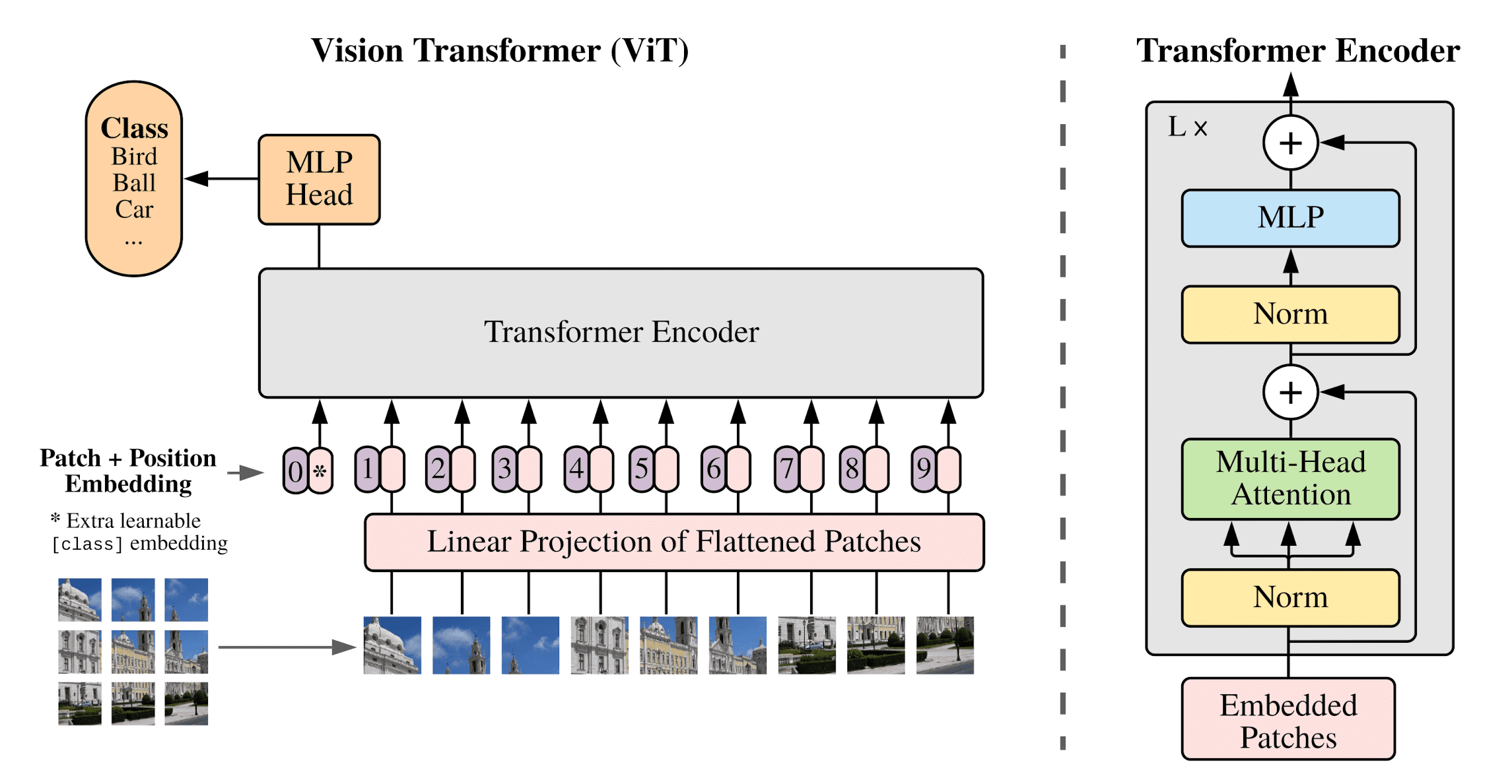
Against this backdrop, models such as the Vision Transformers (ViTs) garner attention for their ability to address this limitation, since they offer flexible sequence-based modeling and hence varying input sequence lengths. This post delves into such approaches of ViTs.
Native Resolution ViT (NaViT)
In language modelling, it is common to bypass limitations of fixed sequence lengths via example packing: tokens from multiple distinct examples are combined in one sequence, which can significantly accelerate training of language models. By treating images as sequences of patches (tokens), Dehghani et al. 2023 show that ViTs can benefit from the same paradigm. Using this technique, ViTs can be trained on images at their “native” resolution, and the authors name this approach NaViT.
Patch n’ Pack: Packing Image Tokens
The packing of examples into sequences, termed as Patch n’ Pack, occurs concurrently with batching. Since there typically is no perfect combination of examples exactly adding up to the fixed length and padding tokens, in NaViT, a straightforward greedy approach is just employed. As shown in the following figure, examples are added to the first sequence with adequate remaining space. Once no additional examples can fit in the remaining space, the sequences are filled with padding tokens, thereby ensuring fixed sequence lengths required for batched operations.
Such simple packing algorithm may result in significant padding, particularly depending on the distribution of input lengths. Various methods, such as bin packing, can mitigate this issue to minimize the padding. In NaViT, the ability to control the resolutions that we sample enables efficient packing by tuning the sequence length, thereby limiting padding to less than 2%.
Since NaViT preserve the native aspect ratio, “effective resolution” is referred to as “resolution” for NaViT from now on. Consequently, images with the same area as a square image with a given resolution are considered equivalent. For example, a resolution of $128$ in NaViT corresponds to the same area of a square $128 \times 128$ image, such as $64 \times 256$, $170 \times 96$, etc., and thus has the same inference cost as regular ViT on $128 \times 128$ images.
Architectural/Training Changes
Example packing of NaViT enables variable resolution images with preserved aspect ratio and offers a significant sample efficiency by enabling more supervision (more examples) within the same compute budget. To support the strategy, the aspects of the data preprocessing and modeling that need to be modified:
- Masked self-attention and masked pooling
To prevent distinct examples attending to & pooling with each other, each token's receptive field should be restricted to the tokens within the same example.
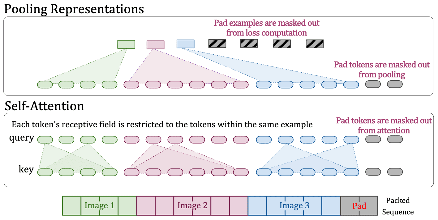
$\mathbf{Fig\ 3.}$ Modified attention and pooling (source: Dehghani et al. 2023)
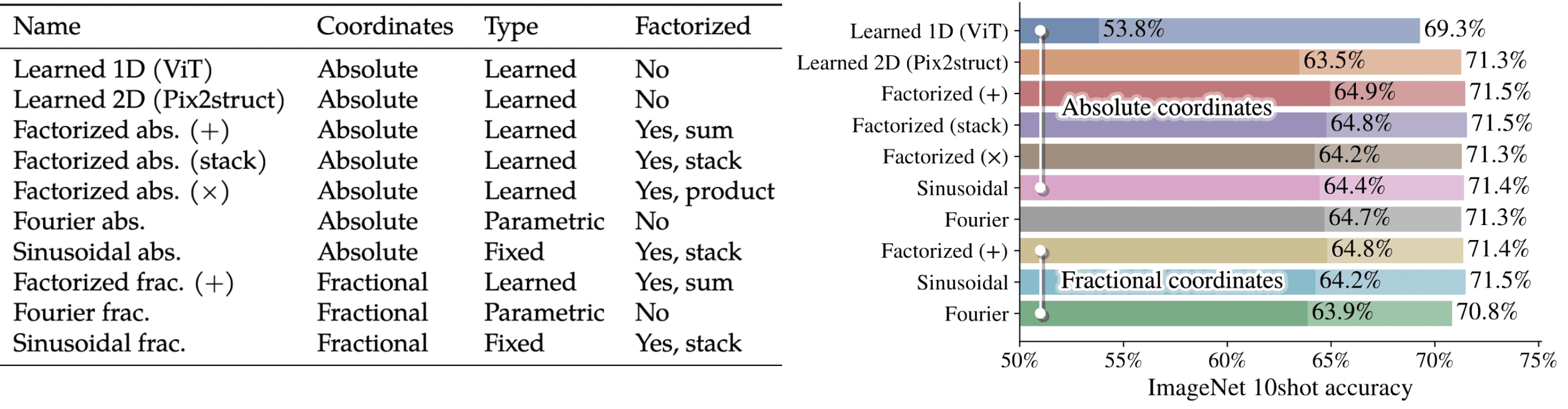
- Factorized & fractional positional embeddings
Given square images of resolution $R \times R$, the original ViT with patch size $P$ learns 1D positional embeddings of length $(R / P)^2$. To support variable aspect ratios and readily extrapolate to unseen resolutions, instead of linear interpolation, NaViT employed factorized fractional positional embeddings, 2D embeddings that decomposes embedding into separate fractional embeddings $\phi_x$ and $\phi_y$ of $x$ and $y$ coordinates. Subsequently, these components are combined using operations such as stacking, summation, or product.
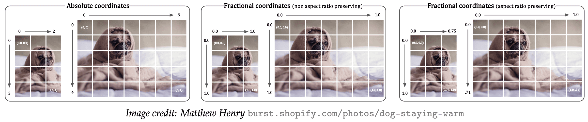
$\mathbf{Fig\ 4.}$ Two schema for positional embeddings
For embedding, two schema are available:-
absolute embeddings $\phi(\mathrm{p}) : [0, \text{maxLen}] \to \mathbb{R}^\mathrm{D}$
- when learned absolute coordinate embeddings are considered, extreme values of $x$ and $y$ must also be observed during training
- necessitates training on images with varied aspect ratios and constrains models generalization.
-
fractional embeddings $\phi(\mathrm{r}) : [0, 1] \to \mathbb{R}^\mathrm{D}$ where $\mathrm{r} = \mathrm{p} / \text{length}$ (relative distance)
- embeddings on fractional coordinates, which are normalized to the actual size of the input image and are obtained by dividing the absolute coordinates $x$ and $y$ above by the number number of columns and rows respectively.
- enables the model to encounter extreme token coordinates throughout training.
And Figure 3 shows the comparison of different embedding choice for $\phi$. It is clear that the factorized approaches outperform both the baseline ViT and the Learned 2D absolute embeddings of size $[\text{maxLen}, \text{maxLen}]$ (Pix2struct). Factorized embeddings are best combined additively (as opposed to stacking or multiplying).
$\mathbf{Fig\ 5.}$ Two schema for positional embeddings
-
absolute embeddings $\phi(\mathrm{p}) : [0, \text{maxLen}] \to \mathbb{R}^\mathrm{D}$
- Continuous Token dropping
Token dropping, random omission of input patches during training, has been developed to accelerate training. However, typically the same proportion of tokens are dropped from all examples; packing enables continuous token dropping, whereby the token dropping rate can be varied per-image. This enables the benefits of faster throughput enabled by dropping while still seeing some complete images, reducing the train/inference discrepancy.
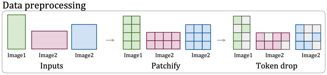
$\mathbf{Fig\ 6.}$ Token dropping (source: Dehghani et al. 2023)
To sample dropping rate $d \in [d_\min, d_\max]$ for each sequence, the paper explored two continuous sampling approaches:- beta distributed dropping rates $$ d = u \times d_{\max} \text{ where } u \sim \mathcal{B}(\alpha, \beta) $$
- resolution-dependent dropping rates $$ d \sim \mathcal{N}_{\textrm{trunc}} (\mu, 0.02) $$ where samples more than two standard deviations away from $\mu$ are rejected. Given input data with sequence lengths from $s_\min$ to $s_\max$, $\mu$ is set according to the minimum and maximum token dropping rates $d_\min$ and $d_\max$, and simply scales linearly with the sequence length $s$ such that $s = s_\min$ has $\mu = d_\min$ and $s = s_\max$ has $\mu = d_\max$: $$ \mu = \frac{s - s_\min}{s_\max - s_\min} (d_\max - d_\min) + d_\min $$
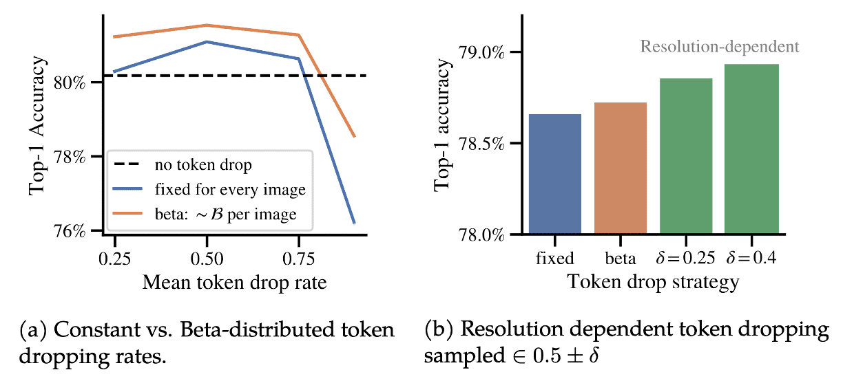
$\mathbf{Fig\ 7.}$ Continuous token dropping strategies enabled by sequence packing improves performance (source: Dehghani et al. 2023)
Or, it is also possible to control the rate with pre-defined schedule. In particular, the paper proposed such that the rate applied for the $n$-th processed image during training is given by: $$ \rho\left(n ; \rho_{\min }, \rho_{\max }, \mu, \tau\right)=\rho_{\min }+\left(\rho_{\max }-\rho_{\min }\right) \times \textrm{sigmoid}\left(\frac{n-\mu}{\tau}\right) $$ where $\rho_\min$, $\rho_\max$ control the minimum and maximum dropping rate applied, and $\mu$ and $\tau$ control the shape of the schedule.
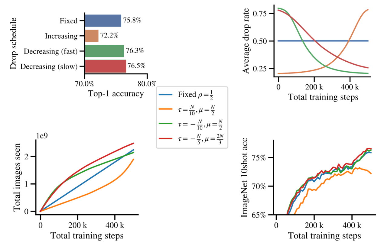
$\mathbf{Fig\ 8.}$ Time-varying token dropping rates improves performance and are easily done with Patch n' Pack. (source: Dehghani et al. 2023)
- Resolution sampling
NaViT allows mixed-resolution training by sampling from a distribution of image sizes, while retaining each images' original aspect ratio. This allows both higher throughput and exposure to large images, yielding substantial improved performance over equivalent ViTs.
For each image, the authors sample $u \sim \mathcal{D}$ of support $[−1, 1]$ with the following choices:- uniform $\mathcal{U} (-1, 1)$
- truncated standard Gaussian $\mathcal{N}_{\text{trunc}, [-1, 1]} (0, 1)$
- Gaussian for lower resolution $\mathcal{N}_{\text{trunc}, [-1, 1]} (-0.5, 1)$
- Gaussian for higher resolution $\mathcal{N}_{\text{trunc}, [-1, 1]} (0.5, 1)$
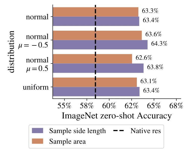
$\mathbf{Fig\ 9.}$ Comparisons between resolution sampling strategies. (source: Dehghani et al. 2023)
Superiority of NaViT
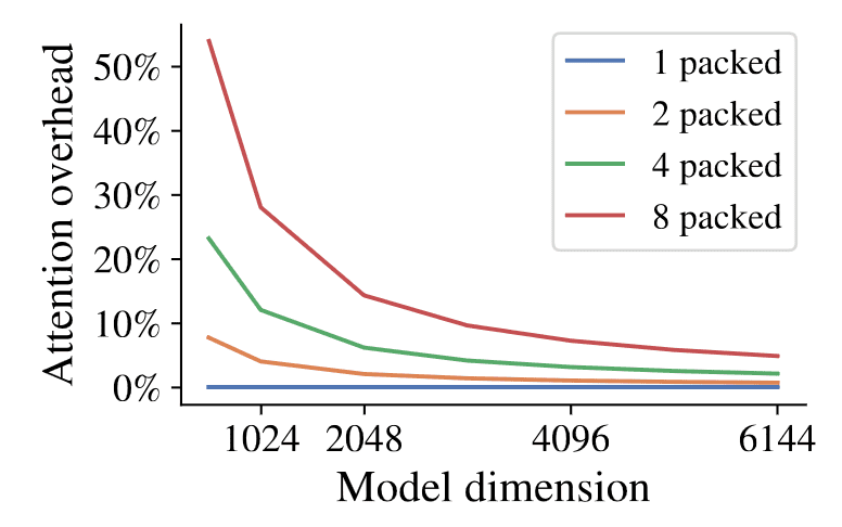
The $\mathcal{O}(n^2)$ cost associated with attention naturally raises concerns when packing multiple images into longer sequences. A plethora of studies aim to mitigate this quadratic cost. However, a more crucial observation is that as we scale transformers, attention becomes a negligible proportion of the overall computation cost.
And Figure 11 depicts the pre-training performance of various NaViT models in comparison to compute-matched ViT baselines. Remarkably, NaViT consistently outperforms ViT while utilizing the same computational budget across different compute and parameter scales. For instance, the performance of the top-performing ViT can be matched by a NaViT with $4 \times$ less compute. Conversely, the computationally lightest NaViT showcased in Figure 11 is $4.9 \times$ more cost-effective than its equivalent ViT counterpart.
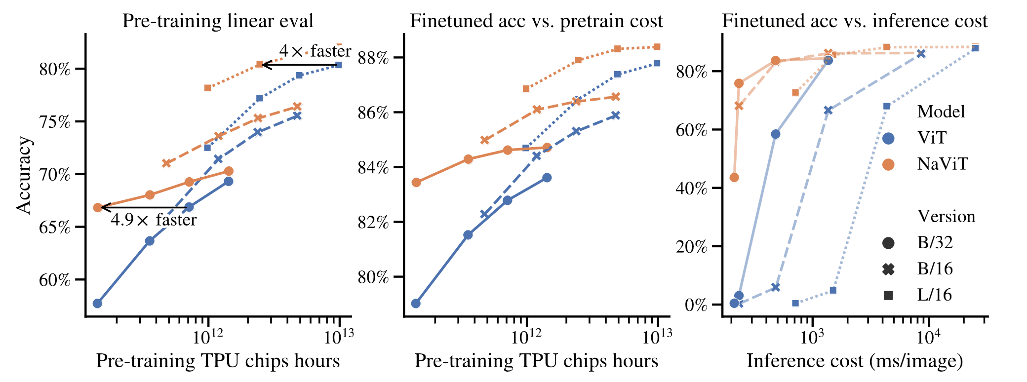
The NaViT models derive benefits from preserved aspect ratios and the capability to evaluate over various resolutions. However, the primary contributor to their success lies in the substantial increase in the number of training examples processed by NaViT within the allocated compute budget. This is accomplished via the combination of sampling multiple variable-resolution examples and token dropping, resulting in variable-sized images efficiently packed into a similar sequence length as the original model.
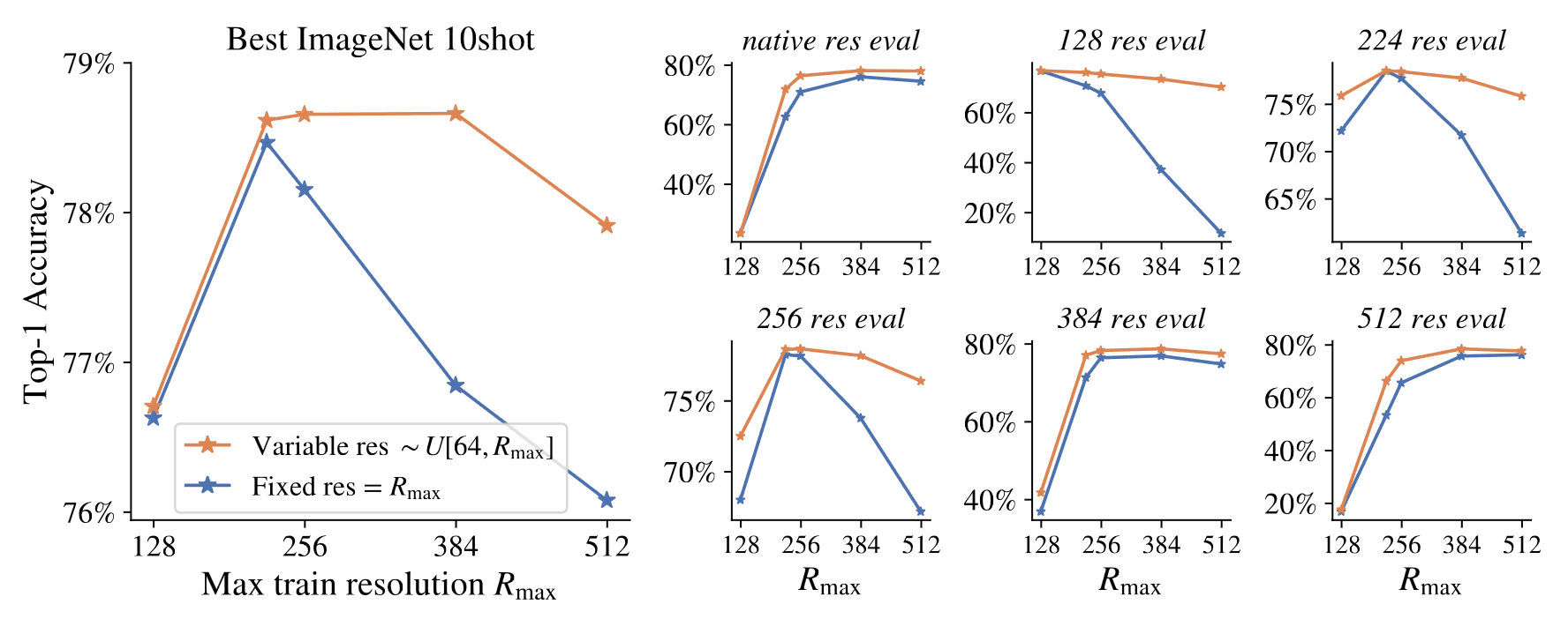
And this is also well-exemplified in the following pre-train experiments. Figure 12 shows a comparison between two NaViT variants trained for the same number of FLOPs but at several different resolutions:
- Fixed resolution model: trained at the native aspect but fixed resolution $R = R_\max$ for different chosen values of $R_\max$.
- Variable resolution model: trained at the variable resolution distributed as $R \sim U(64, R_\max)$.
Variable resolution models outperform models trained at only that resolution. Even in the best case for fixed resolution, where the train and evaluation resolutions are identical, variable resolution matches or outperforms fixed.
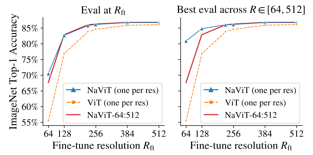
The authors also conducted fine-tuning experiments on NaViT and ViT models at different fixed resolutions, as well as on NaViT at variable resolutions using the ImageNet dataset. Figure 13 illustrates the results of these experiments. Notably, NaViT fine-tuned with variable resolutions (“NaViT 64:512” in the figure) effectively approaches performance comparable to NaViT finetuned at a single resolution, while also outperforming single-resolution ViT. This obviates the need to select a single downstream fine-tuning resolution. Additionally, NaViT fine-tuned at low resolution (64) still achieves good performance when evaluated at higher resolutions, enabling cost-effective adaptation.
ViT with Any Resolution (ViTAR)
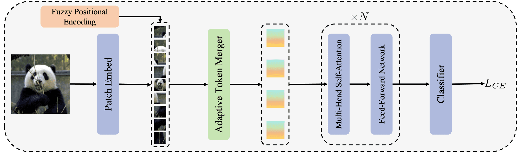
ViTAR, proposed by Fan et al. 2024, processes high-resolution images with low computational burden and exhibits strong resolution generalization capability. It is achieved by two novel modules:
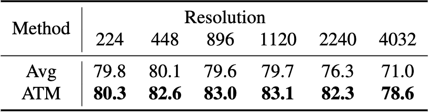
- Adaptive Token Merger (ATM): a simple and effective multi-resolution adaptation module that enhances the model’s exceptional resolution adaptability and low computational complexity for high-resolution images;
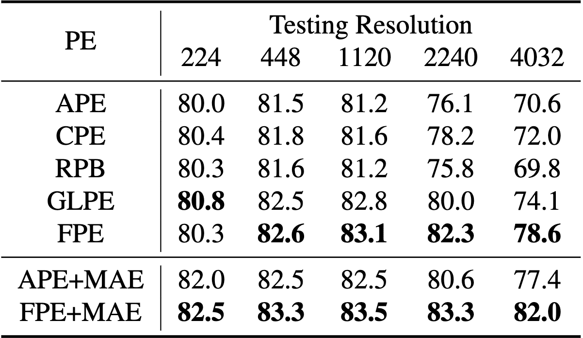
- Fuzzy Positional Encoding (FPE): positional perturbation that transforms precise position perception into a fuzzy perception with random noise, thereby enhancing the model’s resolution adaptability and avoiding overfitting to position at specific resolution;
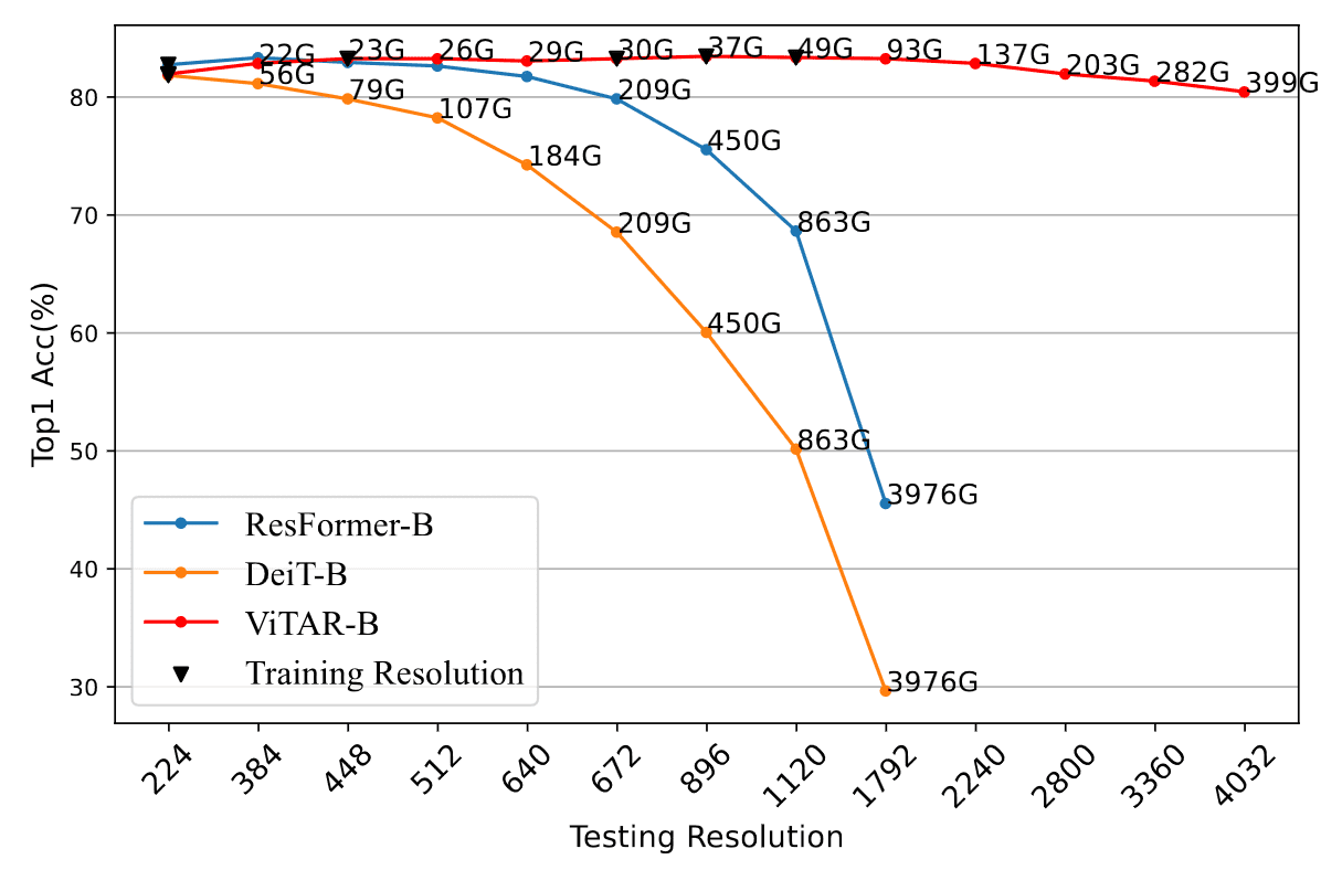
Consequently, ViTAR exhibits the robust generalization to unseen resolutions compared to other ViT models with lower computational cost. Furthermore, ViTAR demonstrates strong performance in downstream tasks including object detection and semantic segmentation, and seamlessly integrates with self-supervised learning methods such as MAE.
Adaptive Token Merger (ATM)
From patch embedding layer, ATM module receives tokens with the shape of $H \times W$ as its input and yields $G_{h} \times G_{w}$ number of merged grid tokens. It initially scatters all tokens onto grids, treating the tokens within a grid as a single unit. It then progressively merges tokens within each unit, ultimately mapping all tokens onto a grid of fixed shape. This procedure yields a collection of what are referred to as “grid tokens”. Subsequently, this set of grid tokens undergoes feature extraction by a sequence of multiple Multi-Head Self-Attention modules. Specifically, it operates as follows:
- Grid Padding and Grid Division
ATM partitions tokens with the shape of $H \times W$ into a grid of size $G_{th} \times G_{tw}$ with total number of $\frac{H}{G_{th}} \times \frac{W}{G_{tw}}$. Practically, $\frac{H}{G_{th}}$ and $\frac{W}{G_{tw}}$ are typically set to $1$ or $2$. That is, we set $G_{th}$ (and $G_{tw}$ also) as following: $$ G_{th} = \begin{cases} \frac{H}{2} & \quad \text{ if } H \geq 2 G_h \\ \frac{\text{GridPadding} (H)}{2} = G_h & \quad \text{ if } 2 G_h > H > G_h \\ G_h & \quad \text{ if } H = G_h \end{cases} $$ The grid padding method is illustrated in Figure 16. It pads with with additional tokens on the right and bottom sides of each grid, ensuring a uniform distribution of padding tokens within each grid. This strategy prevents the occurrence of ineffective grids when common padding methods are employed.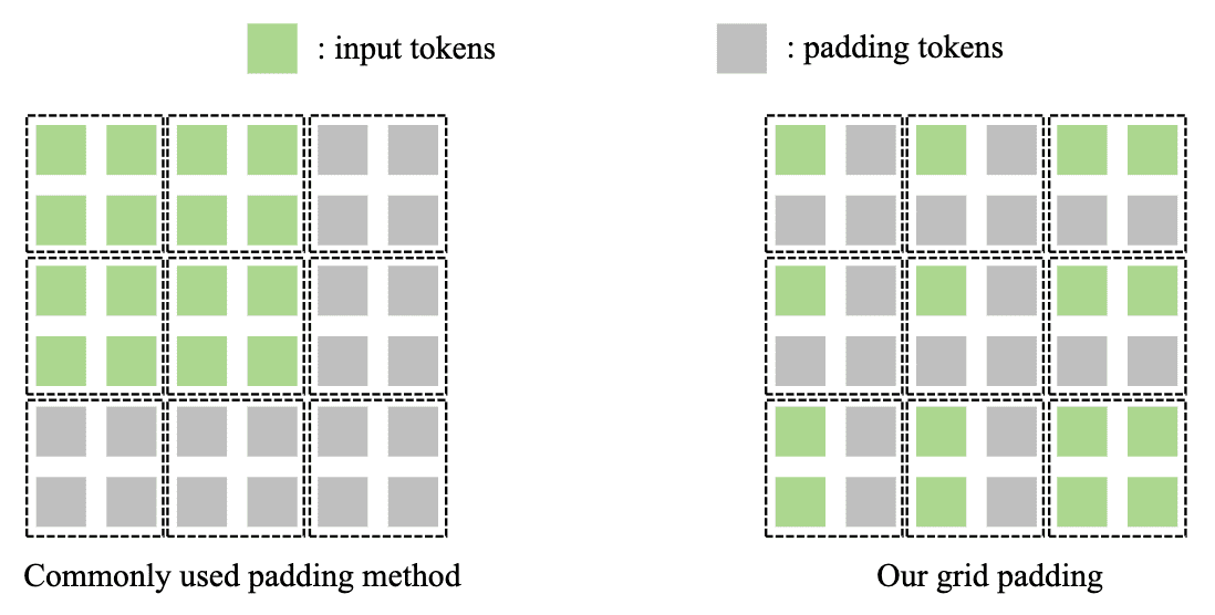
$\mathbf{Fig\ 16.}$ Illustration of Grid Padding (source: Fan et al. 2024)
- Grid Attention
For a specific grid, denote its tokens as a set $\{ x_{ij} \}$ where $0 \leq i < \frac{H}{G_{th}}$ and $0 \leq j < \frac{H}{G_{tw}}$. Obtain the mean token $x_{\text{avg}}$ by average pooling on all $\{ x_{ij} \}$. Considering the mean token as the query, and all $\{x _{ij} \}$ as key and value, we employ cross-attention to merge all tokens within a grid into a single token: $$ \begin{aligned} x_{\text{avg}} & = \text{AvgPool} (\{ x_{ij} \}) \\ \text{GridAttn}(\{ x_{ij} \}) & = x_{\text{avg}} + \text{Attn} (x_{\text{avg}}, \{ x_{ij} \}, \{ x_{ij} \}) \end{aligned} $$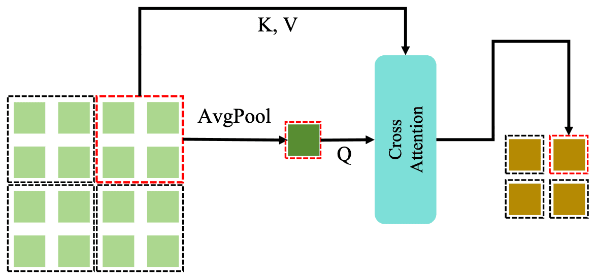
$\mathbf{Fig\ 17.}$ Illustration of Grid Attention (source: Fan et al. 2024)
- Feed-Forward Network (FFN)
After passing through GridAttention, the fused token is directed into a standard Feed-Forward Network to complete channel fusion, thus concluding a single iteration of module. Both GridAttention and FFN undergo multiple iterations and all iterations share the same weights.
ATM module not only enables the model to seamlessly adapt to a range of input resolutions, but also leads to low computational complexity when dealing with high-resolution images by token fusion.
Fuzzy Positional Encoding (FPE)
During the model training, typical positional encodings often provide precise location information to the model. Instead, FPE only supplies the model with fuzzy positional information by shifting the positional information $(i, j)$ within a certain range; $(i + s_1, j + s_2)$ where $s_1, s_2 \sim U[-0.5, 0.5]$.
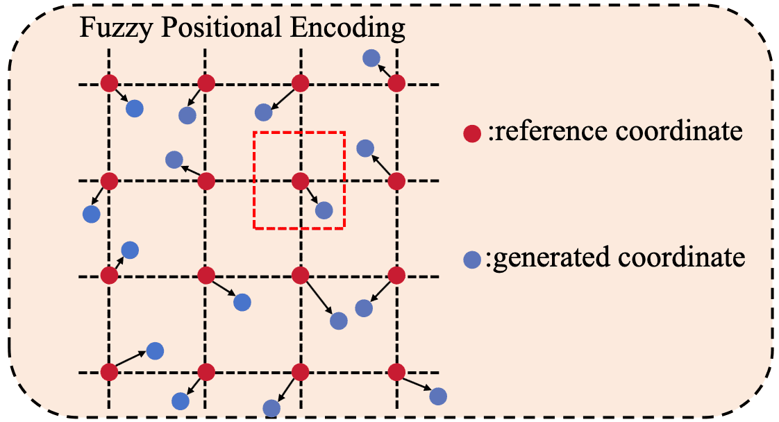
During inference, the precise positional encoding is used instead of the Fuzzy Positional Encoding. And when a modification in the input image resolution occurs, it performs an interpolation on the learned positional embeddings. Owing to the use of fuzzy positional encoding during the training phase, the model might have encountered and used any interpolated positional encoding. Consequently, the model gains robust positional resilience, leading to strong performance when faced with inputs of unseen resolutions.
Reference
[1] Dehghani et al. “Patch n’ Pack: NaViT, a Vision Transformer for any Aspect Ratio and Resolution”, NeurIPS 2024
[2] Fan et al. “ViTAR: Vision Transformer with Any Resolution”, arxiv:2403.18361
Leave a comment