
[DB] Relational Language
The relational model is the primary data model for commercial data-processing applications. It attained its primary position because of its simplicity, which eases the job of the programmer, compared to earlier data models such as the network model or the hierarchical model.
Structure of Relational Databases
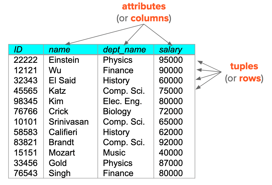
A relational database consists of a collection of tables, each of which is assigned a unique name. In general, a row in a table represents a relationship among a set of values.
- In the relational model, the term relation is used to refer to a table, whilst the term tuple is used to refer to a row.
- Similarly, the term attribute refers to a column of a table.
- Denoted as $A_1, \cdots, A_n$.
- A relation schema consists of a list of attributes and their corresponding domains.
- Denoted as $R=(A_1, \cdots, A_n)$.
- e.g.
instructor = (ID, name, dept_name, salary)
- The term relation instance refers to a specific instance of relation schema $R$, i.e., containing a specific set of rows.
- Denoted as $r(R)$.
- An element $t$ of a relation $r$ is called a tuple.
- The domain of the attribute refers to the set of allowed values for each attribute.
- e.g. the domain of
salaryattribute is the set of all possible salary values - Attribute values are normally required to be atomic, i.e., elements of the domain are considered to be indivisible units and do not allow set values.
- The special value null is a member of every domain, indicating that the value is “unknown”.
- e.g. the domain of
- Relations are unordered, like sets in mathematics.
Keys
We must have a way to specify how tuples within a given relation are distinguished; no two tuples in a relation are allowed to have exactly the same value for all attributes.
Let $K \subseteq R$, where $R$ is a relational schema for the relation $r$.
-
Superkey
$K$ is a superkey of $R$ if value for $K$ are sufficient to identify a unique tuple of each possible relation instance $r(R)$.- i.e., $\forall t_1,t_2 \in R : t_1 \neq t_2 \implies t_1.K \neq t_2.K$
- e.g. in
instructorrelation,IDand(ID, name)are superkeys.
-
Candidate key
A superkey $K$ is a candidate key if $\lvert K \rvert$ is at its minimum value.- several distinct sets of attributes could serve as candidate key
- e.g. in
instructorrelation,IDis candidate key.
-
Primary key
Only one of the candidate keys is selected to be the primary key.- Usually the most efficient one in terms of computation cost is chosen.
- Chosen by the database designer with care as the principal means of identifying tuples within a relation.
- Chosen such that its attribute values are never, or are very rarely, changed.
- Also referred to as the primary key constraints.
Next, we consider another type of constraint on the contents of relations. Let $A_i$ be an attribute of relations $r_i$.
-
A foreign-key constraint from attribute(s) $A_1$ of relation $r_1$ to the primary-key $A_2$ of relation $r_2$ states that on any database instance, the value of $A_1$ for each tuple in $r_1$ must also be the value of $A_2$ for some tuple in $r_2$.
- i.e., $\forall t_1 \in R_1 : \exists t_2 \in R_2 \quad \text{ s.t. } \quad t_1.A_1=t_2.A_2$
-
Motivation
Consider the attributedept_nameof theinstructorrelation. It would not make sense for a tuple ininstructorto have a value fordept_namethat does not correspond todepartmentin the department relation.
-
Attribute set $A_1$ is called foreign key from $r_1$, referencing $r_2$.
- $r_1$: referencing relation;
- $r_2$: referenced relation;
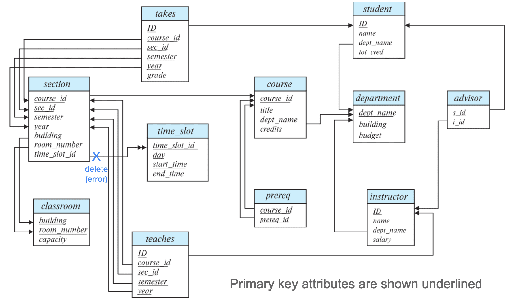
A database schema, along with primary key and foreign-key constraints, can be depicted by schema diagrams.
Relational Query Languages
A query language is a language in which a user requests information from the database. Query languages can be categorized as:
-
Imperative query language
- the user instructs the system to perform a specific sequence of operations on the database to compute the desired result
-
Functional (Procedural) query language
- the computation is expressed as the evaluation of functions that may operate on data in the database or on the results of other functions; functions are side-effect free, and they do not update the program state.
- it can be also referred to as procedural query language, languages based on procedure (function) invocations. However, the term is also widely used to refer to imperative languages.
-
Declarative query language
- the user describes the desired information without giving a specific sequence of steps or function calls for obtaining that information.
Relational Algebra
The relational algebra is a procedural query language consisting of a set of operations that take one or two relations as input and produce a new relation as their result.
- Six basic operators
- select: $\sigma$
- project: $\Pi$
- union: $\cup$
- set difference: $-$
- Cartesian product: $\times$
- rename: $\rho$
1. Select $\sigma$
The select operation selects tuples that satisfy a given predicate
- Notation: $\sigma_p(r)$
- $p$ is called the selection predicate
- e.g., select those tuples of the instructor relation where the instructor is in the “Physics” department
- Query: $\sigma_{\textrm{dept_name=“Physics”}}(\textrm{instructor})$
- Result:
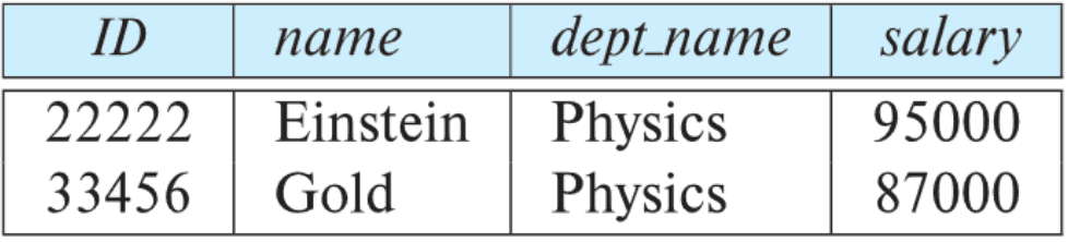
- Comparisons uses $=$, $\neq$, $>$, $\geq$, $<$, $\leq$ in the selection predicate.
- Predicates are combined using connectives; $\wedge$, $\vee$, $\neg$.
- The select predicate can also include comparisons between two different attributes.
2. Projection $\Pi$
The (unary) projection operator $\Pi$ returns its argument relation, with certain attributes removed.
- Notation: $\Pi_{A_1, \cdots, A_k}(r)$, where $A_i$'s are attribute names and $r$ is a relation name.
- e.g., eliminate the dept_name attribute of instructor
- Query: $\Pi_{\textrm{ID},\textrm{name},\textrm{salary}}(\textrm{Instructor})$
- Result:
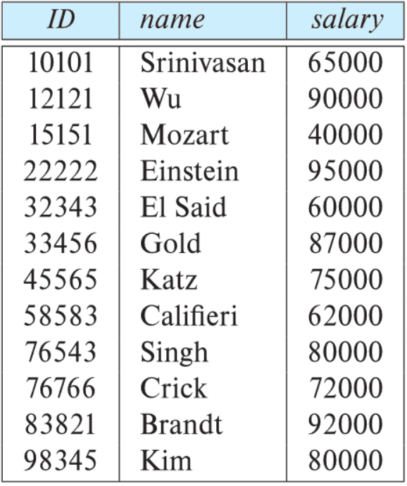
- The result is defined as the relation of $k$ columns obtained by erasing the columns that are not listed.
- Duplicate rows removed from the result, since relations are sets.
3. Cartesian Product $\times$
The (binary) Cartesian operator $\times$ combines information from any two relations. As a result, it constructs a tuple of the result out of each possible pair of tuple from each relation and one from the teaches relation.
- Notation: $r_1 \times r_2$, where $r_j$ are relations.
- e.g. the Cartesian product of the relations instructor and teaches
- Query: $\textrm{Instructor} \times \textrm{Teaches}$
- Result:
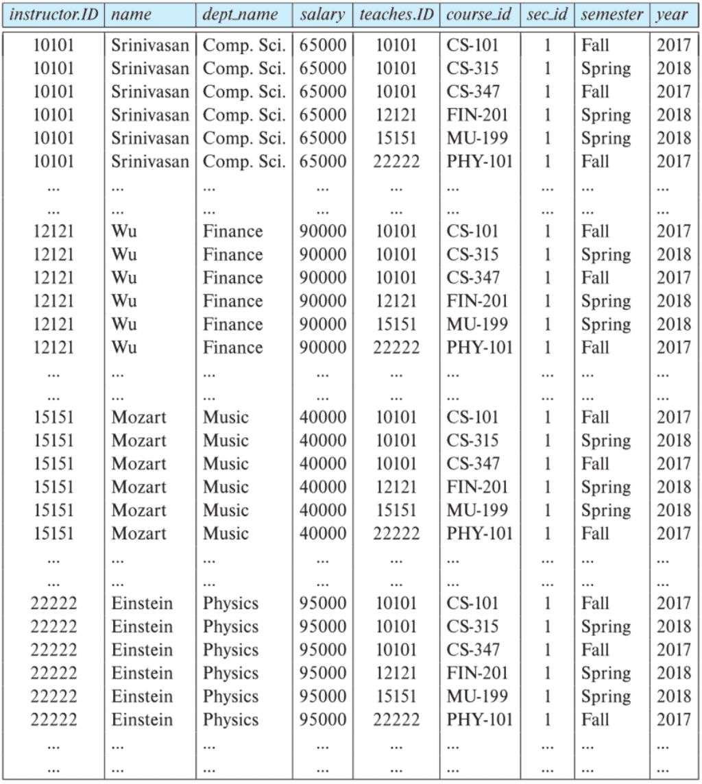
- To distinguish between attribute appears in both relations, attach the name of the source relation to the name of the attribute
- e.g. $\textrm{Instructor}.\textrm{ID}$, $\textrm{Teaches}.\textrm{ID}$
- Duplicate rows removed from the result, since relations are sets.
Join $\bowtie$
The Cartesian product $r_1 \times r_2$ associates every tuple of $r_1$ with every tuple of $r_2$. Hence, most of the resulting rows have the redundant information. To get only desired tuples that pertain to our predicate $p$, we may write
\[\sigma_p (r_1 \times r_2)\]The composition of a cartesian product followed by a selection operation is called join operator $\bowtie$ defined as follows:
\[r \bowtie_p s = \sigma_p (r \times s)\]- e.g. $\textrm{Instructor} \bowtie_{\textrm{Instructor}.\textrm{ID} = \textrm{Teaches}.\textrm{ID}} \textrm{Teaches}$
- Result:
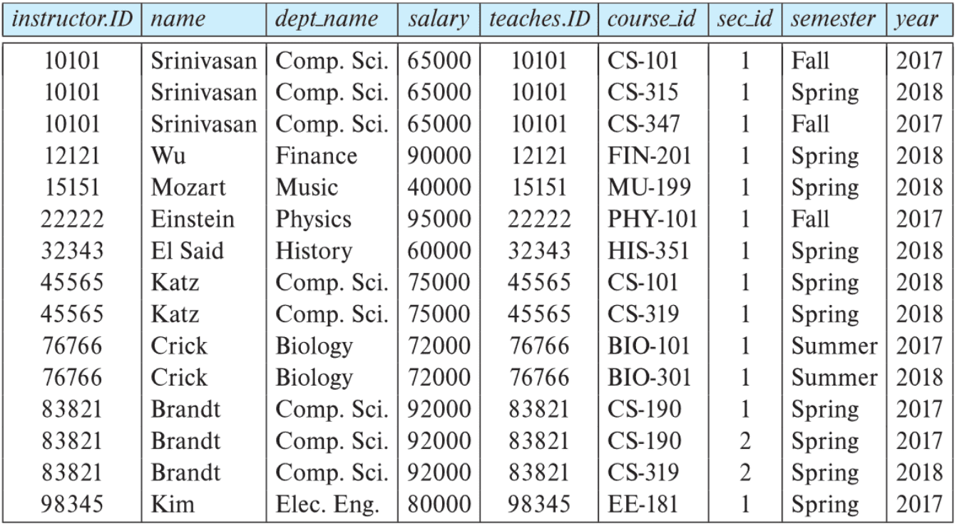
- It returns only those tuples that satisfy some predicate $p$, among all possible combinations of tuples from the two relations.
- It does not belong to the six basic operations.
4. Union $\cup$
The (binary) union operator $\cup$ combines two relations and returns all tuples that are present in at least one of the relations. Two relations must satisfy the condition.
- Notation: $r_1 \cup r_2$, where $r_j$ are relations.
- e.g. find all courses taught in the Fall 2017 semester, or in the Spring 2018 semester, or in both
- Query: $\prod_{\textrm{courseID}} (\sigma_{\textrm{semester}=\textrm{"Fall"} \wedge \textrm{year}=2017} (\textrm{Section})) \cup \prod_{\textrm{courseID}} (\sigma_{\textrm{semester}=\textrm{"Spring"} \wedge \textrm{year}=2018} (\textrm{Section}))$
Two relations must satisfy the conditions to be valid:
- $r_1$ and $r_2$ must have the same arity (same number of attributes)
- The attribute domains must be compatible (e.g., the 2nd column of $r_1$ deals with the same type of values as does the 2nd column of $r_2$)
Intersection $\cap$
The (binary) intersection operator $\cap$ combines two relations and returns all tuples that are present in both the relations.
- Notation: $r_1 \cap r_2$, where $r_j$ are relations.
- e.g. find all courses taught in both the Fall 2017 semester and the Spring 2018 semester
- Query: $\prod_{\textrm{courseID}} (\sigma_{\textrm{semester}=\textrm{"Fall"} \wedge \textrm{year}=2017} (\textrm{Section})) \cap \prod_{\textrm{courseID}} (\sigma_{\textrm{semester}=\textrm{"Spring"} \wedge \textrm{year}=2018} (\textrm{Section}))$
Two relations must satisfy the conditions to be valid:
- $r_1$ and $r_2$ must have the same arity (same number of attributes)
- The attribute domains must be compatible (e.g., the 2nd column of $r_1$ deals with the same type of values as does the 2nd column of $r_2$)
5. Set-Difference $-$
The (binary) set-difference operator $-$ combines two relations and returns all tuples that are in one relation but are not in another.
- Notation: $r_1 - r_2$, where $r_j$ are relations.
- e.g. find all courses taught in the Fall 2017 semester, but not in the Spring 2018 semester
- Query: $\prod_{\textrm{courseID}} (\sigma_{\textrm{semester}=\textrm{"Fall"} \wedge \textrm{year}=2017} (\textrm{Section})) - \prod_{\textrm{courseID}} (\sigma_{\textrm{semester}=\textrm{"Spring"} \wedge \textrm{year}=2018} (\textrm{Section}))$
Two relations must satisfy the conditions to be valid:
- $r_1$ and $r_2$ must have the same arity (same number of attributes)
- The attribute domains must be compatible (e.g., the 2nd column of $r_1$ deals with the same type of values as does the 2nd column of $r_2$)
Assignment $\leftarrow$
The assignment operator $\leftarrow$ assigns a relational algebra expression to a temporary relation variable. It works similar as the assignment operation in programming languages. Note that it does not provide any additional power to the algebra.
- Notation: $x \leftarrow E$, where $x$ is a name and $E$ is a relational algebra expression.
- e.g. Find all instructors in any of the Physics or Music departments: $$ \begin{aligned} & \textrm{Physics} \leftarrow \sigma_{\textrm{dept_name} = \textrm{"Physics"}} (\textrm{Instructor}) \\ & \textrm{Music} \leftarrow \sigma_{\textrm{dept_name} = \textrm{"Music"}} (\textrm{Instructor}) \\ & \textrm{Physics} \cup \textrm{Music} \\ \end{aligned} $$
- With the assignment operation, a query can be written as a sequential program consisting of a series of assignments followed by an expression whose value is displayed as the result of the query.
6. Rename $\rho$
Relations have their name, whereas the results of relational-algebra expressions do not; it is useful to be able to give them names. The (unary) rename operator $\rho$ assigns a name to the results of relational algebra expressions, and returns the result of the expression $E$ under the given name $x$, and with the attributes renamed to $A_1, \cdots, A_n$.
- Notation: $\rho_{x(A_1,\cdots,A_k)}(E)$ where $x$ is a name, $A_i$'s are attributes, and $E$ is a relational algebra expression.
- e.g. Find the ID and name of those instructors who earn more than the instructor whose ID is 12121.
- Query: $\prod_{i.\textrm{ID}, i.\textrm{name}} ( \sigma_{i.\textrm{salary} > w.\textrm{salary}} (\rho_i (\textrm{Instructor}) \times \sigma_{w.\textrm{ID} = 12121} (\rho_w (\textrm{Instructor}))) )$
- Rename compared with Assignment
- Naming a relation: this function can be used to give a name to a result relation; therefore, in this aspect, the rename operation may be equivalent to the assignment operation
- Renaming a relation and its attributes: the rename operation can change the names of attributes, whereas the assignment operation cannot
Remarks
-
Composition of Relational Operations
The result of a relational-algebra operation is a relation, and therefore relational-algebra operations can be composed together into a relational-algebra expression.- e.g. find the names of all instructors in the “Physics” department
- Query: $\Pi_{\textrm{dept_name}} (\sigma_{\textrm{dept_name}=\textrm{"Physics"}} (\textrm{Instructor}))$
-
Equivalent Queries
There is more than one way to write a query in relational algebra.- e.g., find information about courses taught by instructors in the Physics department with a salary greater than 90,000
- Query 1: $\sigma_{\textrm{dept_name}=\textrm{"Physics"} \wedge \textrm{Salary} > 90000} (\textrm{Instructors}) $
- Query 2: $\sigma_{\textrm{dept_name}=\textrm{"Physics"}} ( \sigma_{\textrm{Salary} > 90000} (\textrm{Instructors}) )$
- e.g., find information about courses taught by instructors in the Physics department
- Query 1: $\sigma_{\textrm{dept_name}=\textrm{"Physics"}} (\textrm{Instructor} \bowtie_{\textrm{Instructor}.\textrm{ID} = \textrm{Teaches}.\textrm{ID}} (\textrm{Teaches}) )$
- Query 2: $(\sigma_{\textrm{dept_name}=\textrm{"Physics"}} (\textrm{Instructor})) \bowtie_{\textrm{Instructor}.\textrm{ID} = \textrm{Teaches}.\textrm{ID}} \textrm{Teaches}$
- e.g., find information about courses taught by instructors in the Physics department with a salary greater than 90,000
Reference
[1] Silberschatz, Abraham, Henry F. Korth, and Shashank Sudarshan. “Database system concepts.” (2011).
Leave a comment