[DB] Complex Data Types

The relational model is very widely used for data representation for a large number of application domains. A fundamental requirement of the relational model is that data values be atomic: multivalued, composite, and other complex data types are prohibited by the core relational model. However, in many instances, the constraints on data types enforced by the relational model present more challenges than solutions. In this post, we explore several non-atomic data types that are widely used, including semi-structured data, object-based data, textual data, and spatial data.

Semi-Structured Data

• Many applications require storage of complex data, whose schema changes often.
• The relational model’s requirement of atomic data types may be too strict;
  • e.g., storing set of interests as a set-valued attribute of a user profile may be simpler than normalizing it
• Data exchange can benefit greatly from semi-structured data.
  • Exchange can be between applications, or between back-end and front-end of an application
  • Web-services are widely used today, with complex data fetched to the front-end and displayed using a mobile app or JavaScript
• JSON and XML are widely used semi-structured data models

Features of Semi-Structured Data Models

• Flexible Schema
  • Wide column representation: each tuple is allowed to have a different set of attributes, and new attributes can be added at any time.
  • Sparse column representation: schema has a fixed but large set of attributes, where each tuple may store only a subset of attributes.
• Multivalued Data Types
  • Many databases allow the storage of multi-valued data types as attribute values.
  • Sets, Multisets
    • e.g., set of interests {'basketball', 'La Liga', 'cooking', 'anime', 'jazz'}
  • Key-value map (or just map)
    • A set of key-value pairs;
    • e.g., {(brand, Apple), (ID, MacBook Air), (size, 13), (color, silver)}
    • Operations on maps: put(key, value), get(key), delete(key)
• Arrays
  • Widely used for scientific and monitoring applications.
  • e.g., readings taken at regular intervals can be represented as array of values instead of (time, value) pairs
    • [5, 8, 9, 11] instead of {(1, 5), (2, 8), (3, 9), (4, 11)}
• Array database: a database that provides specialized support for arrays
  • e.g., compressed storage, query language extensions, etc.
  • Oracle GeoRaster, PostGIS, SciDB, etc.

Nested Data Types

• Many data representations allow attributes to be structured, directly modeling composite attributes in the E-R model.
  • e.g. name attribute with components first_name and last_name
• All of these data types represent a hierarchy of data types, and that structure leads to the use of the term nested data types.
• Two widely used data representations that allow values to have complex internal structures and that are flexible in that values are not forced to adhere to a fixed schema:
  • JavaScript Object Notation (JSON);
  • Extensible Markup Language (XML);

JSON

• Textual representation widely used for data exchange
  • Example of JSON data

      {
          "ID": "22222",
          "name": {
              "firstname": "Albert",
              "lastname": "Einstein"
          },
          "deptname": "Physics",
          "children": [
              {"firstname": "Hans", "lastname": "Einstein" },
              {"firstname": "Eduard", "lastname": "Einstein" }
          ]
      } 
    

  • Objects are key-value maps, i.e., sets of (attribute name, value) pairs
  • Arrays are also key-value maps (from an offset to a value)
• JSON is ubiquitous in data exchange today;
  • Especially being widely used for Web services
    • Most modern applications are architected around on Web services to store and retrieve data
• SQL extensions are available for
  • JSON data types for storing JSON data;
  • Extracting data from JSON objects using path expressions;
    • e.g., v->ID, or v.ID
  • Generating JSON from relational data;
    • e.g., json_build_object(‘ID’, 12345, ‘name’, ‘Einstein’)
  • Creating JSON collections using aggregation;
    • e.g., json_agg aggregate function in PostgreSQL, which returns a JSON array
  • Syntax varies greatly across databases (see this document for SQLite3);
• JSON is verbose;
  • takes up more storage space for the same data, and parsing the text to retrieve required fields can be very CPU-intensive.
  • Compressed representations such as BSON (Binary JSON) is widely used for efficient data storage.

XML

• XML uses tags to markup the text
  • e.g.

    <course>
        <course_id> CS-101 </course_id>
        <title> Intro. to Computer Science </title>
        <dept_name> Comp. Sci. </dept_name>
        <credits> 4 </credits>
    </course> 
  

• Tags make the data self-documenting in that a human can understand.
• Tags can be used to create hierarchical structures, which is not possible with the relational model.
• XQuery language developed to query nested XML structures.
  • Not widely used currently;
• SQL extensions to support XML
  • Storing XML data as XML data types;
  • Generating XML data from relational data;
  • Extracting data from XML data types;
    • Path expressions

Knowledge Representation

Representation of human knowledge has long been a goal of the artificial intelligence community. A variety of models were proposed for this task, with varying degrees of complexity; these could represent facts as well as rules about facts. With the growth of the web, a need arose to represent extremely large knowledge bases, with potentially billions of facts.

RDF and Knowledge Graphs

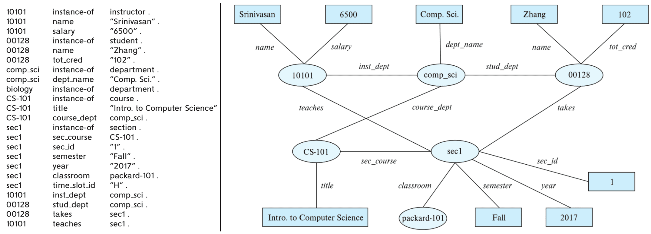
The Resource Description Framework (RDF) is a simplified representation standard based on the E-R model.

• It represents data by a set of triples (subject, predicate, object);
  • e.g., (NBA-2019, winner, Raptors), (Washington-DC, capital-of, USA), etc.
• Modeling objects having attributes and relationships with other objects
  • Like the ER model, but with a flexible schema
  • (ID, attribute-name, value)
  • (ID1, relationship-name, ID2)
• Having a natural graph representation, referred to as knowledge graph

$\mathbf{Fig\ 1.}$ RDF representation and Knowledge graph

Note that RDF triples represent binary relationships. Then, how can $n$-ary relationships be represented?

• Approach 1. reification: creating an artificial entity and linking to each of the $n$ entities;
  • e.g., (Barack Obama, president-of, USA, 2008-2016) can be represented as
    • (e1, person, Barack Obama), (e1, country, USA), (e1, president-from, 2008), (e1, president-till, 2016)
• Approach 2. using quads instead of triples, with context entities
  • e.g., (Barack Obama, president-of, USA, c1)
    • (c1, president-from, 2008), (c1, president-till, 2016)

RDF is widely used as knowledge base representation, such as DBPedia, Yago, Freebase, WikiData, etc. In addition, there are a very large number of domain-specific knowledge graphs. Linked Open Data project aims to connect different knowledge graphs to allow queries to span databases.

Querying RDF: SPARQL

SPARQL is a query language designed to query RDF data.

• The language is based on triple patterns, which look like RDF triples but may contain variables;
  • e.g., ?cid title "Intro. to Computer Science", ?sid course ?cid, etc.
  • ? indicates a variable.
• Example: a complete SPARQL query

  • retrieve names of all students who have taken a section whose course is titled "Intro. to Computer Science"

      SELECT ?name 
      WHERE {
          ?cid title "Intro. to Computer Science". /* '.' indicates the end of a triple pattern*/
          ?sid course ?cid.
          ?id takes ?sid.
          ?id name ?name. 
      }
    

    • The shared variables between these triples enforce a join condition between the tuples matching each of these triples.

Object Orientation

• Object-relational data model provides a richer type system, with complex data types and object orientation
• Applications are often written in object-oriented programming languages, such as Java, Python, or C++.
  • Need to store and fetch data from databases
  • The type system of the object-oriented programming language does not match the relational type system supported by databases
  • Switching between an imperative language and SQL is troublesome
• Three approaches are used in practice for integrating object-orientation with database systems:
  • Build an object-relational database, adding object-oriented features to a relational database;
  • Automatically convert data between the programming language model and the relational model; data conversion specified by object-relational mapping;
  • Build an object-oriented database system that natively supports object-oriented data and direct access from the programming language;

Object-Relational Database Systems

How can object-oriented features be added to relational database systems?

User-Defined Types

Object extensions to SQL allow creation of structured user-defined types, references to such types, and tables containing tuples of such types.

• User-Defined Types

  • e.g.

      CREATE TYPE Person
          (ID VARCHAR (20) PRIMARY KEY,
          name VARCHAR (20),
          address VARCHAR (20)) 
          REF FROM (ID);  /* More on this later */
      CREATE TABLE people OF Person;
    

• Table types

  • e.g.

      CREATE TYPE interest AS TABLE (
          topic VARCHAR (20),
          degree_of_interest INT ); 
      CREATE TABLE users (
          ID VARCHAR (20),
          name VARCHAR (20),
          interests interest );
    

• Array & Multiset data types also supported by many databases
  • Syntax varies by database

Type & Table Inheritance

• Type Inheritance

  • e.g. we may want to store extra information in the database about people who are students and about people who are teachers:

      CREATE TYPE Student UNDER Person
          (degree VARCHAR (20));
      CREATE TYPE Teacher UNDER Person
          (salary INTEGER);
    

• Table Inheritance
  • it allows a table to be declared as a sub-table of another table and corresponds to the E-R notion of specialization/generalization;

  • e.g.

      /* PostgreSQL */
      CREATE TABLE students
          (degree VARCHAR (20))
          INHERITS people;
      CREATE TABLE teachers
          (salary integer)
          INHERITS people; 
    
      /* Oracle */
      CREATE TABLE people OF Person;
      CREATE TABLE students OF Student
          UNDER people;
      CREATE TABLE teachers OF Teacher
          UNDER people; 
    

Reference Types

An existing primary-key value can be used to reference a tuple by including the REF FROM clause in the type definition.

• Creating reference types

  • e.g.

      CREATE TYPE Person
          (ID VARCHAR (20) PRIMARY KEY,
          name VARCHAR (20),
          address VARCHAR (20))
          REF FROM (ID);
      CREATE TABLE people of Person; 
      CREATE TYPE Department (
          dept_name VARCHAR (20),
          head REF (Person) SCOPE people);
      CREATE TABLE departments OF Department;
    

  • SCOPE clause above completes the definition of the foreign key from Departments.head to the people relation.

  • System generated references can be retrieved using subqueries

      SELECT REF (p)
      FROM People AS p
      WHERE ID = '12345'
    

• References are dereferenced in SQL:1999 bypath expressions ->

    SELECT head->name, head->address
    FROM departments; 
  

?? 책 다시 읽기 및 강의

Object-Relational Mapping

Object-Relational Mapping (ORM) systems allow:

• a programmer to define mapping between programming language objects and database tuples;
• automatic creation of database tuples upon creation of objects;
• automatic update/delete of database tuples when objects are update/deleted;
• interface to retrieve objects satisfying specified conditions;
• tuples in database are queried, and object are created from the tuples;

Advantage

• Any of a number of databases can be used to store data, with exactly the same high-level code.
  • ORMs hide minor SQL differences between databases from the higher levels.
  • Migration from one database to another is thus relatively straightforward when using an ORM
  • In contrast, SQL differences can make such migration significantly harder if an application uses SQL to communicate with the database.

Disadvantage

• ORM systems can suffer from significant performance inefficiencies for bulk database updates, as well as for complex queries that are written directly in the imperative language.
  • It is possible to update the database directly, bypassing the ORM system, and to write complex queries directly in SQL in cases where such inefficiencies are discovered.

But the benefits of ORMs exceed the drawbacks for many applications, and ORM systems have seen widespread adoption in recent years.

Textual Data

Textual data consists of unstructured text. The term information retrieval generally refers to the querying of unstructured textual data.

Keyword Queires

Information retrieval systems support the ability to retrieve documents with some desired information, typically described by a set of keywords.

• Information retrieval: querying of unstructured data
  • Simplest form: given query keywords, retrieve documents containing all the keywords
  • More advanced models rank the documents according to their relevance
  • Today, keyword queries return many types of information as answers
    • e.g., a query "Son Heung-min" returns information about early life, club career, …

Relevance Ranking

Relevance ranking> is essential since there are usually many documents matching keywords.

TF-IDF

The word term refers to a keyword occurring in a document, or given as part of a query. And term trequency (TF), the relevance of a term $t$ to a document $d$, can be measured by using informations such as number of occurences, abstract, author list ,etc.

The natural intuition is that the ‘relative’ number of occurrences of the term in the document serves as measure of its relevance:

\[\mathrm{TF}(d, t) = \log \left( 1 + \frac{n(d, t)}{n(d)}\right)\]

where $n(d)$ denotes the number of term occurrences in the document and $n(d, t)$ denotes the number of terms $t$ in the document $d$.

A query $Q$ may contain multiple keywords. The relevance of a document to a query with two or more keywords is estimated by combining the relevance measures of the document for each keyword. To combine their relevance measure effectively, weights can be assigned to terms using the inverse document frequency (IDF), defined as:

\[\mathrm{IDF}(t) = \frac{1}{n(t)}\]

where $n(t)$ denotes the number of documents containing term $t$. Then, the relevance $r(d, Q)$ of a document $d$ to a set of terms $Q$ is defined as:

\[r(d, Q) = \sum_{t \in Q} \mathrm{TF}(d, t) \times \mathrm{IDF}(t)\]

This measure can be further refined if the user is permitted to specify weights $w(t)$ for terms in the query. The above approach of using term frequency and inverse document frequency as a measure of the relevance of a document is called the TF–IDF approach.

Hyperlinks

Hyperlinks between documents can be used to decide on the overall importance of a document, independent of the keyword query; for example, documents linked from many other documents are considered more important.

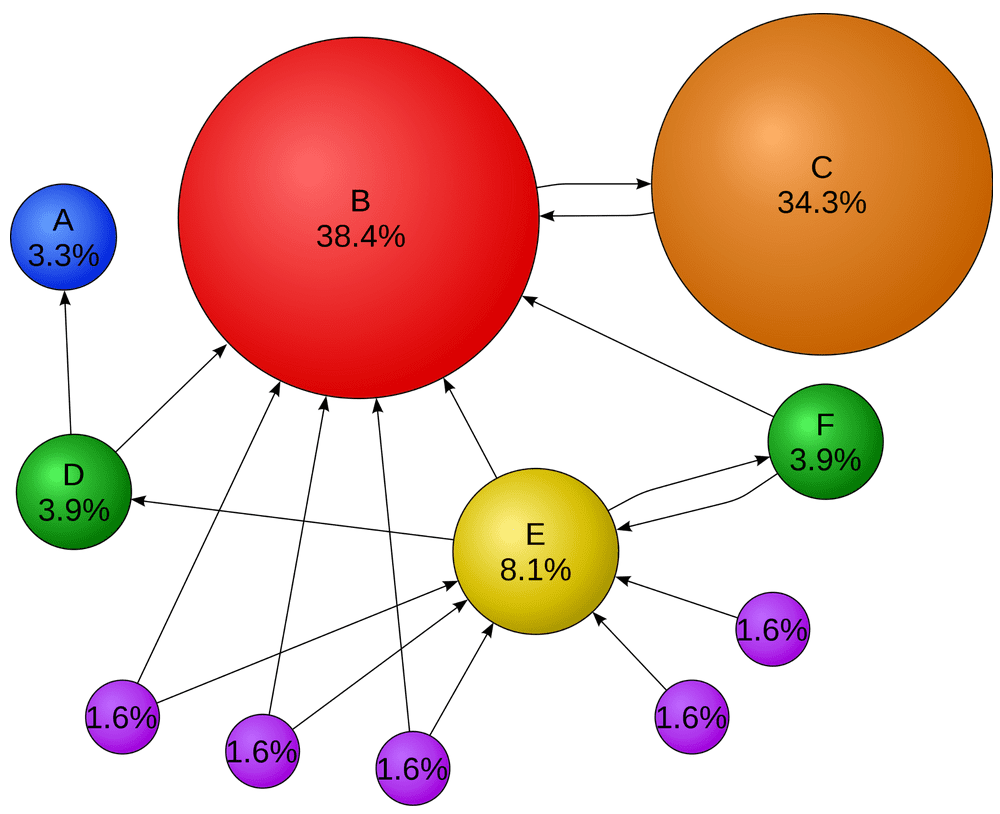
PageRank

A measure of popularity/importance based on hyperlinks to pages, developed by Google.

• Rationale
  • Pages hyperlinked from many pages should have a higher PageRank
  • Pages hyperlinked from the pages with a higher PageRank should have a higher PageRank
    • Formalized by the random walk model

$\mathbf{Fig\ 2.}$ PageRank (source: Wikipedia)

• Formulation
  • Let $T[i, j]$ be the probability that a random walker who is on page $i$ will click on the link to page $j$.
    • Assuming all links are equal, $T[i, j] = \frac{1}{N_i}$ where $N_i$ denotes number of links out of page $i$.

  • Then, PageRank $P[j]$ for each page $j$ can be defined as

    \[P[j] = \frac{\delta}{N} + (1-\delta) \sum_{i=1}^N (T[i, j] * P[i])\]
    • $N$ denotes total number of pages
    • $\delta$ is a constant usually set to $0.1$
• Solver
  • the definition of PageRank is circular, but can be solved as a set of linear equations; ㅁ simple iterative technique works well
    • Initialize all $P[j] = 1/N$;
    • In each iteration, apply $P[j] = \frac{\delta}{N} + (1-\delta) \sum_{i=1}^N (T[i, j] * P[i])$ to update $P$
    • Stop iteration when changes are small, or a certain limit (e.g., 30 iterations) is reached

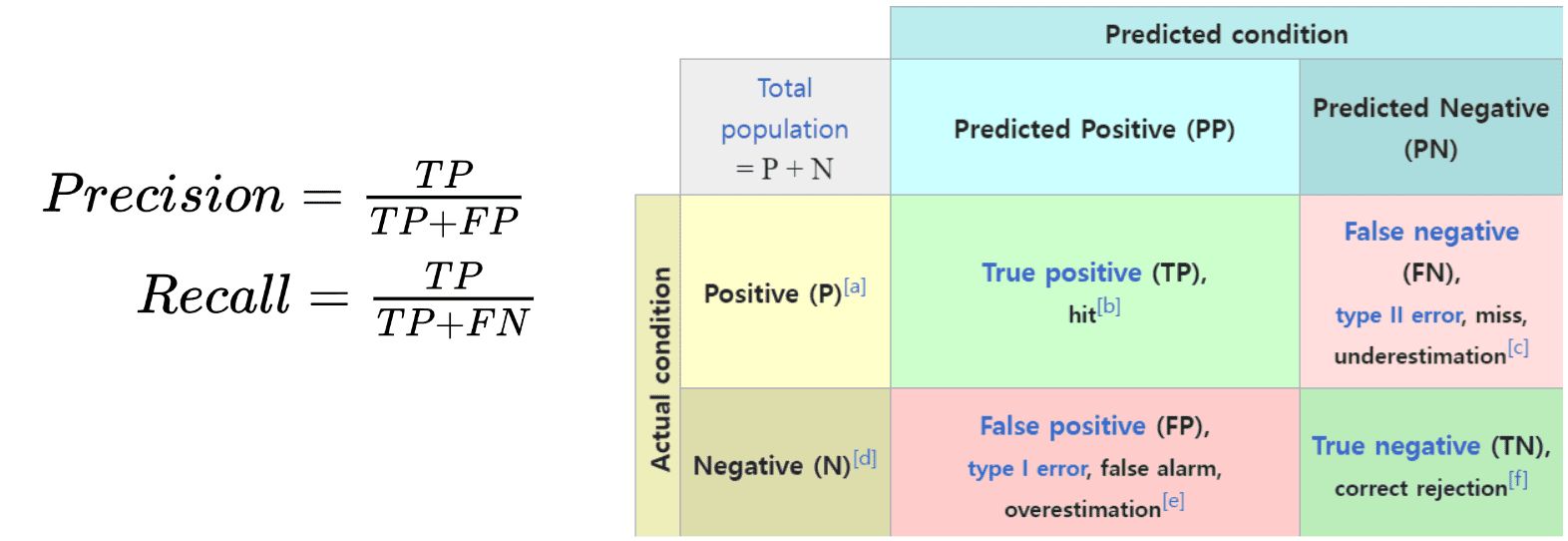
Retrieval Effectiveness

To measure how well an information-retrieval system is able to answer queries:

• Precision: what percentage of returned results are actually relevant;
• Recall: what percentage of relevant results are returned;
  • At some number of answers, e.g., precision@10, recall@10

$\mathbf{Fig\ 3.}$ Measuring Retrieval Effectiveness: Confusion Matrix (source: Wikipedia)

Spatial Data

Spatial data support in database systems store information related to spatial locations, and support efficient storage, indexing, and querying of spatial data. Two types of spatial data are particularly important:

• Geographic data
  • e.g., road maps, land-usage maps, topographic elevation maps, political maps showing boundaries, land-ownership maps, etc.
  • Geographic information systems (GISs) are special-purpose databases tailored for storing geographic data
  • A round-earth coordinate system can be used, e.g., (latitude, longitude, elevation)
• Geometric data
  • design information about how objects are constructed
  • e.g., designs of buildings, aircraft, layouts of integrated-circuits
  • based on 2 or 3 dimensional Euclidean space with $(X, Y, Z)$ coordinates

Geometric Information

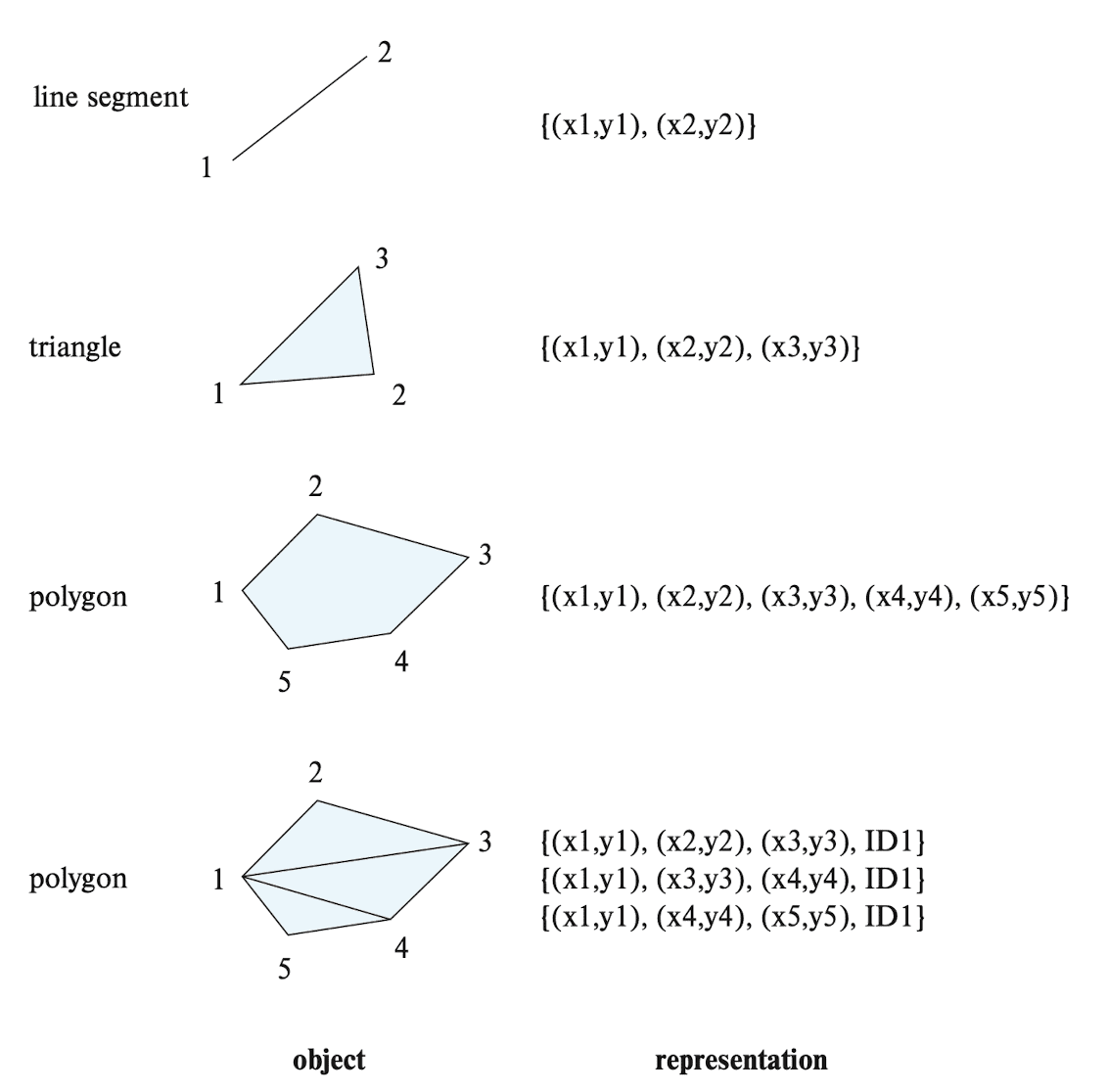
Various geometric constructs can be represented in a database, in a normalized fashion.

• line segment
  • can be represented by the coordinates of its endpoints
• polyline (linestring)
  • consists of connected sequence of line segments
  • can be represented by list containing the coordinates of the endpoints of the segments, in sequence
  • In order to approximate a curve, it is divided into a series of segments
    • Useful for two-dimensional features such as roads
• polygon
  • can be represented by a list of vertices in order
    • The list of vertices specifies the boundary of a polygonal region
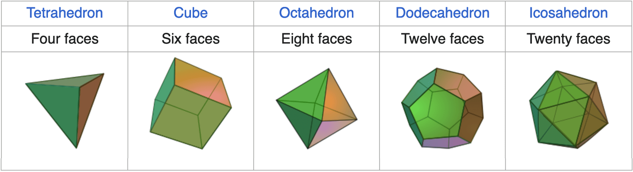
  • can also be represented as a set of triangles (triangulation)

$\mathbf{Fig\ 4.}$ Representation of geometric constructs

Representation of points and line segments in 3D is similar to 2D, except that points have an extra $z$ component.

• Arbitrary polyhedra can be represented by tetrahedrons, which is analogous to how triangulating polygons
• Geometry and geography data types are supported by many databases, e.g., SQL Server and PostGIS
  • Point, Linestring, Curve, Polygons
    • LINESTRING(1 1, 2 3, 4 4)
    • POLYGON((1 1, 2 3, 4 4, 1 1))
  • Collections
    • multipoint, multilinestring, multicurve, multipolygon
  • Type conversions
    • ST_GeometryFromText() and ST_GeographyFromText()
  • Operations
    • ST_Union(), ST_Intersection(), …

$\mathbf{Fig\ 5.}$ 3D geometric constructs (source: Wikipedia)

Design Databases

For large designs, such as the design of a large-scale integrated circuit or the design of an entire airplane, it may be impossible to hold the complete design in memory. Designers of object-oriented databases were motivated in large part by the database requirements of CAD systems.

• Design components are represented as objects (generally geometric objects); the connections between the objects indicate how the design is structured
  • Simple two-dimensional objects
    • points, lines, triangles, rectangles, polygons
  • Complex two-dimensional objects
    • construction from simple objects via union, intersection, and difference operations
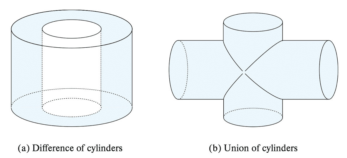
  • Complex three-dimensional objects
    • construction from simpler objects such as spheres, cylinders, and cuboids, by union, intersection, and difference operations (See $\mathbf{Fig\ 7.}$)
• Wireframe models can also represent 3D surfaces as a set of simpler objects. (See $\mathbf{Fig\ 6.}$)

$\mathbf{Fig\ 6.}$ Example of wireframe model (source: Dassault Systèmes and PGBS)

$\mathbf{Fig\ 7.}$ Example of complex 3D objects

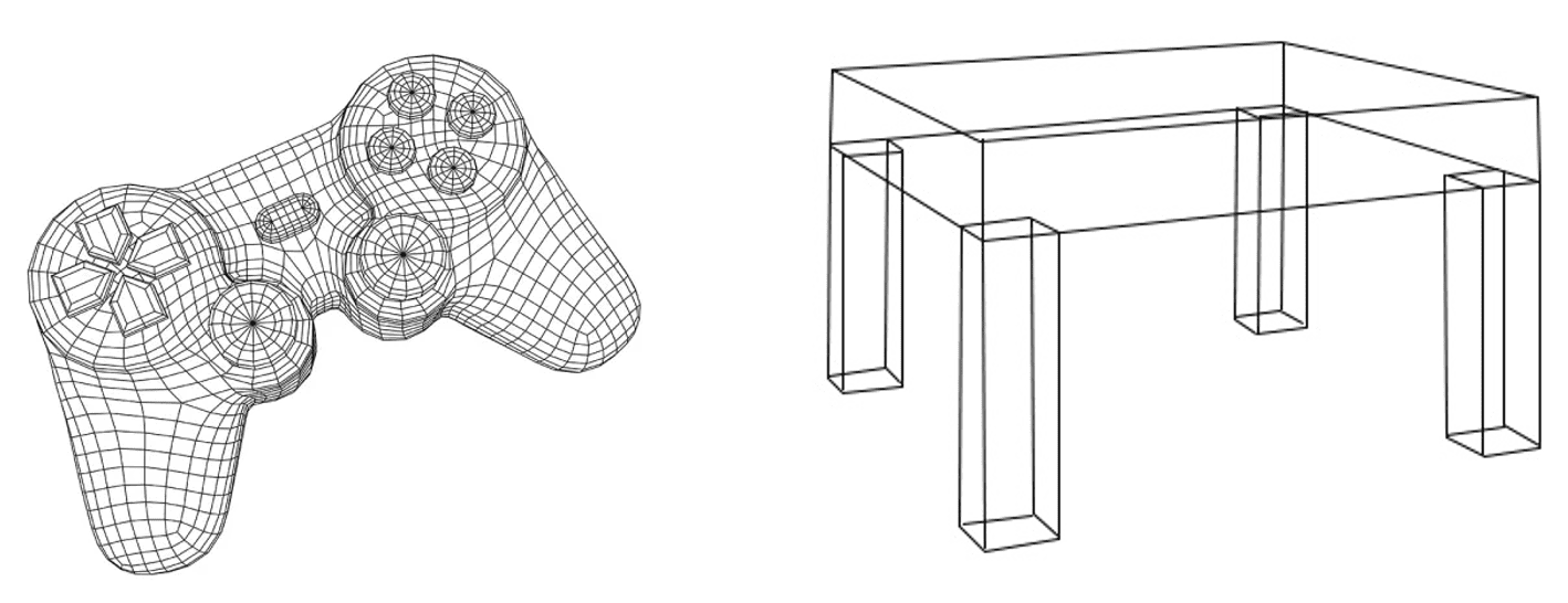
• Design databases also store non-spatial information about objects.
  • e.g., construction material, color, etc.
• Spatial integrity constraints are important
  • e.g., “pipes should not be in the same location” to prevent interference errors

Geographic Data

Geographic data are spatial in nature but differ from design data in certain ways. Maps and satellite images are typical examples of geographic data. Maps may provide not only location information — about boundaries, rivers, and roads, for example — but also much more detailed information associated with locations, such as elevation, soil type, land usage, and annual rainfall.

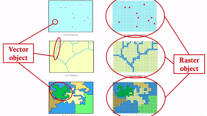
Geographic data can be categorized into two types:

• Raster data
  • consist of bitmaps or pixel maps, in two or more dimensions
  • e.g., satellite image of cloud cover, where each pixel stores the cloud visibility in a particular area
    • Additional dimensions might include the temperature at different altitudes at different regions, or measurements taken at different points in time
  • Design databases generally do not store raster data
• Vector data
  • constructed from basic geometric objects: points, line segments, triangles, and other polygons in two dimensions, and cylinders, spheres, cuboids, and other polyhedrons in three dimensions
  • The vector format is often used to represent map data
    • Roads can be considered as two-dimensional and represented by polylines
    • Some features, such as rivers, may be represented either as complex curves or as complex polygons, depending on whether their width is relevant
    • Geographic features such as regions and lakes can be depicted as complex polygons

$\mathbf{Fig\ 8.}$ Comparison of raster and vector data (source: FME)

Spatial Queries

There are numerous types of queries that involve spatial locations.

• Region queries deal with spatial regions, e.g., ask for objects that lie partially or fully inside a specified region;
  • e.g., PostGIS: ST_Contains(), ST_Overlaps(), …
• Nearness queries request objects that lie near a specified location;
  • e.g. find all restaurants that lie within a given distance of a given point
• Nearest neighbor queries, given a point or an object, find the nearest object that satisfies given conditions;
• Spatial graph queries request information based on spatial graphs
  • e.g., shortest path between two points via a road network
• Spatial join of two spatial relations with the location playing the role of join attribute
  • queries that compute intersections or unions of regions

In general, queries on spatial data may have a combination of spatial and nonspatial requirements. For instance, we may want to find the nearest restaurant that has vegetarian selections and that charges less than $10 for a meal.

Reference

[1] Silberschatz, Abraham, Henry F. Korth, and Shashank Sudarshan. “Database system concepts.” (2011).