[DB] Vector Databases

The revolution of AI skyrocket data complexity and high-dimensional information, rendering traditional databases inadequate for efficiently handling and querying intricate datasets. Against this backdrop, vector database has emerged as a solution to the challenges posed by the ever-expanding data landscape.

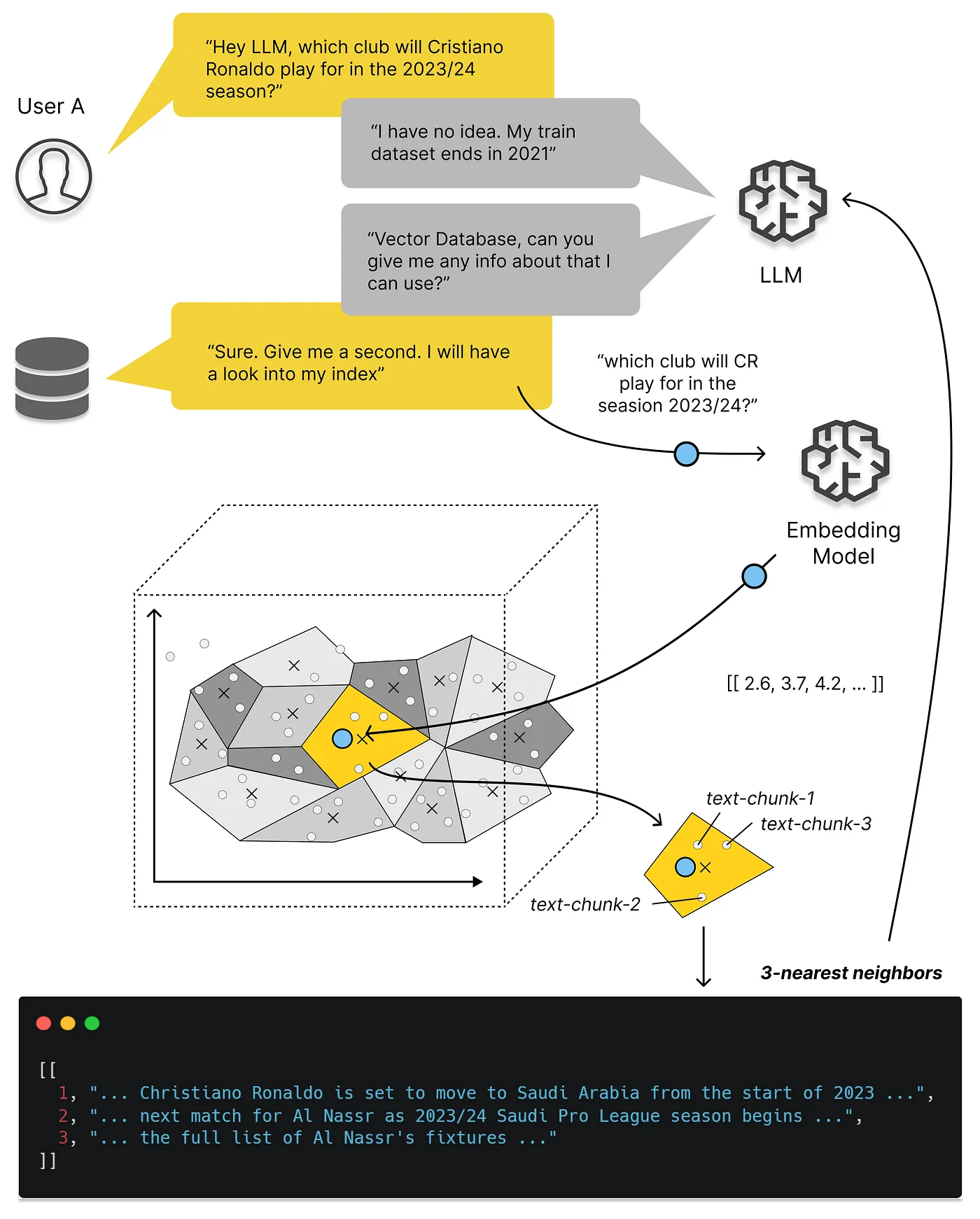
For instance, a large language model (LLM) is AI model capable of executing various natural language processing (NLP) tasks based on pre-trained knowledge. However, LLMs are susceptible to hallucinations due to their lack of domain-specific knowledge. Here, vector databases are an essential technology that can mitigate this issue by furnishing LLMs with domain-specific, up-to-date, or confidential private data.

$\mathbf{Fig\ 1.}$ Why we need Vector Stores for LLM apps (source: Dominik Polzer)

Vector Databases

Vector database indexes and stores vector embeddings for fast retrieval and similarity search, with capabilities like CRUD operations, metadata filtering, horizontal scaling, and serverless. It is designed to handle data where each entry is represented as a vector in a multi-dimensional space, possessing a wide range of information such as numerical features, embeddings from text or images, and even complex data like molecular structures.

Vector databases store data by using vector embeddings. Each entity is allocated a vector that encapsulates diverse attributes or features of that object, and these vectors are structured in such a way that similar objects have vectors that are proximate to each other in the vector space, whereas disparate objects have vectors that are distant apart. For example, in a music streaming application, songs could be represented as vectors using embeddings that capture musical features such as tempo, genre, and instrumental composition.

The significance of vector databases lies in their capabilities and applications:

• Efficient similarity search
  • Vector databases excel in similarity searches, facilitating the retrieval of vectors that closely resemble a given query vector.
• High-dimensional data
  • Vector databases are designed to handle high-dimensional data with greater efficacy, rendering them suitable for applications such as natural language processing, and computer vision.
• Machine learning and AI
  • Vector embeddings capture the pivotal attributes of the data and can be used for diverse tasks, encompassing clustering, classification, and anomaly detection, etc.

General Pipeline

In traditional databases, we are usually querying for rows in the database where the value usually exactly matches our query. However, in vector databases, we apply a similarity metric to find a vector that is the most similar to our query, called Approximate Nearest Neighbor (ANN).

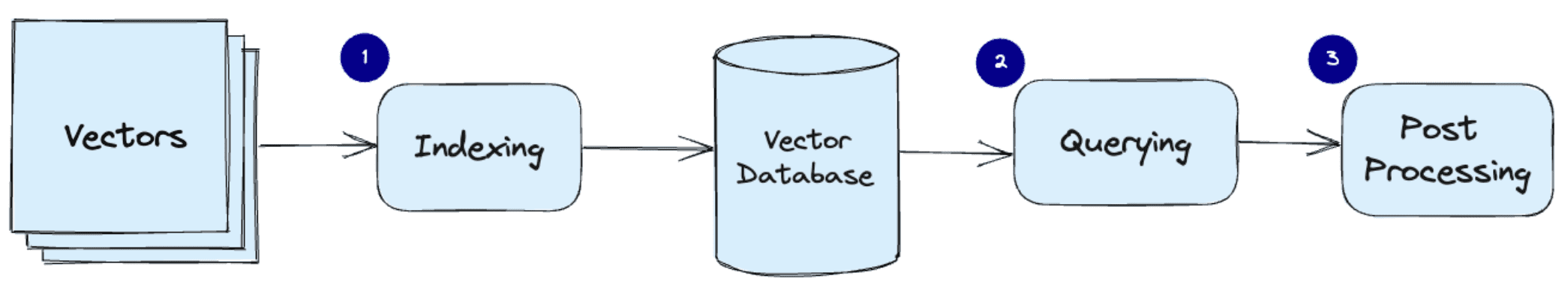
The search algorithms including hashing, quantization, or graph-based search, are assembled into a pipeline that provides fast and accurate retrieval of the neighbors of a queried vector. The general pipeline of vector database is given as follows:

1. Indexing
   The vector database indexes vectors using an algorithm such as product quantization (PQ), locality-sensitive hashing (LSH), or hierarchical navigable small world (HNSW).
2. Querying
   The vector database compares the indexed query vector to the indexed vectors in the dataset to find the nearest neighbors with the similarity metric used by that index.
3. Post-processing
   The vector database retrieves the final nearest neighbors from the dataset, post-processes them to return the final results. (optional)

$\mathbf{Fig\ 2.}$ Pipeline of Vector database (source: pinecone)

Indexing Algorithms

Several algorithms can facilitate the creation of a vector index. Their common goal is to enable fast querying by creating a data structure that can be traversed quickly.

Random Projection

One of the simplest idea approach to creating an index is random projection, where high-dimensional vector embeddings are projected to a lower-dimensional space using a random projection matrix.

$\mathbf{Fig\ 3.}$ Random projection (source: Pinecone)

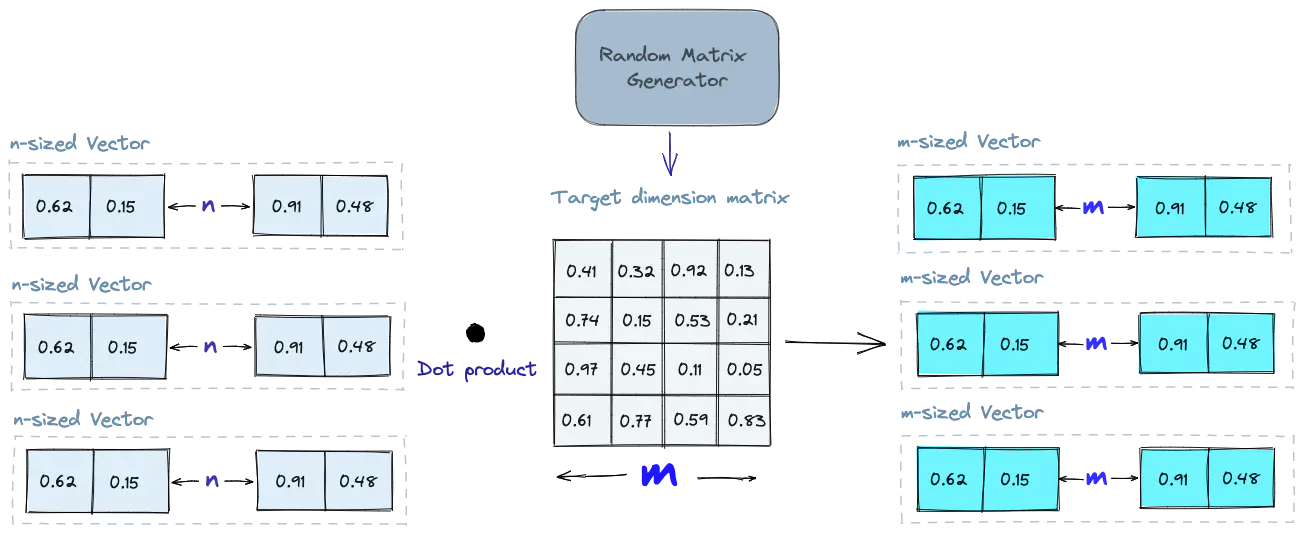
When querying, we utilize the same projection matrix to map the query vector onto a lower-dimensional space. We then compare the projected query vector to the projected vectors in the database. With reduced dimensionality, the search process is markedly faster than searching through the entire high-dimensional space.

Product Quantization (PQ)

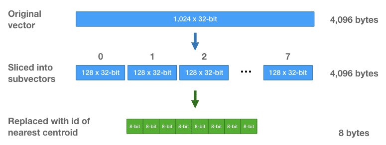
Product quantization (PQ) decomposes the original vector into smaller segments, simplifies each segment by creating a representative code for it, and then recombines the segments. This process retains the essential information necessary for similarity operations.

$\mathbf{Fig\ 4.}$ Product Quantization (PQ) (source: Chris McCormick)

Specifically, the overall algorithm of product quantization can be decomposed into four intermediate steps:

1. Split
   The vectors are decomposed into segments.
2. Train
   The algorithm generates a pool of potential codes that can be assigned to a vector. (e.g., Centroids of k-means clustering)
3. Encode
   The algorithm assigns a specific code to each segment.
4. Query
   When querying, the algorithm decomposes the vectors into sub-vectors and quantizes them using the same codebook. It then utilizes the indexed codes to identify the vectors nearest to the query vector.

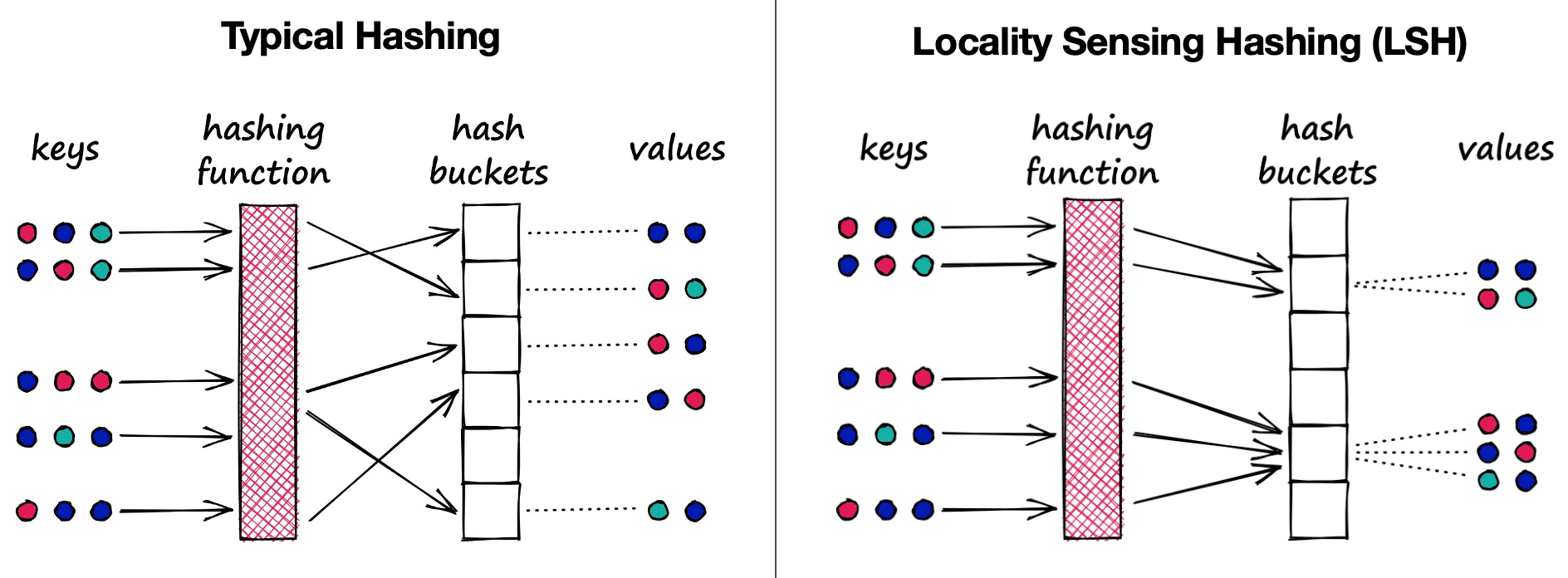
Locality-Sensitive Hashing (LSH)

Locality-Sensitive Hashing (LSH) maps similar vectors into buckets using a set of hashing functions. To find the nearest neighbors for a given query vector, it utilizes the same hashing functions used to bucket similar vectors into hash tables. Then the bucket of query vector is compared with the other vectors in that same table to find the closest matches. This method is significantly faster than searching the entire dataset, as there are far fewer vectors in each hash table.

Note that locality-sensitive hashing is a fuzzy hashing technique that hashes similar input items into the same buckets with high probability. Therefore, there is a key disctinction between typical hash functions and LSH functions. A typical hash function aims to place different values, regardless of their similarity, into separate buckets, whereas a LSH function aims to place similar values into the same buckets.

$\mathbf{Fig\ 5.}$ Typical Hashing v.s. Locality-Sensitive Hashing (source: Pinecone)

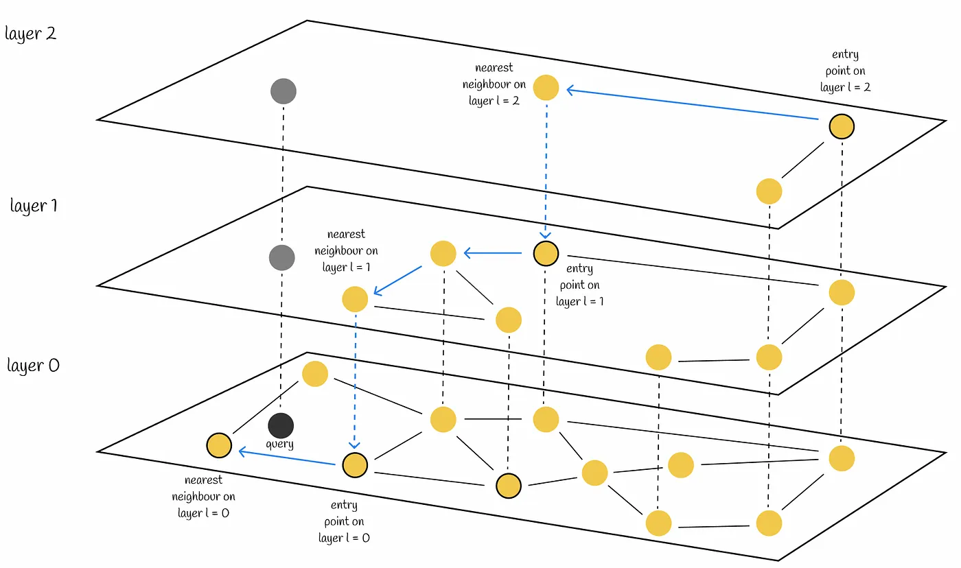
Hierarchical Navigable Small World (HNSW)

Hierarchical Navigable Small World (HNSW) constructs a hierarchical, graph-like structure where each node represents a set of vectors, and the edges between the nodes denote the similarity between vectors. The algorithm initiates by generating a set of nodes, each containing a small number of vectors. This process may be executed randomly or through vector clustering, where each cluster forms a node. Subsequently, the algorithm evaluates the vectors within each node and establishes edges between the node and those nodes housing the most similar vectors.

When querying an HNSW index, the algorithm utilizes this graph to traverse through the structure. The search starts from the highest layer and and iterates downwards, with the local nearest neighbor being greedily discovered among the nodes at each layer. Finally, the nearest neighbor found at the lowest layer serves as the answer to the query.

$\mathbf{Fig\ 6.}$ Searching in Hierarchical Navigable Small World (HNSW) (source: Vyacheslav Efimov)

Querying Metrics

The similarity measures constitute the pivotal components of querying in vector databases, employed to compare the vectors stored within the database and find those most proximate to a given query vector. The following are the most prevalent metrics for quantifying similarity between two vectors:

• cosine similarity: measures the cosine of the angle between two vectors in a vector space

\[\mathrm{d}(\mathbf{u}, \mathbf{v}) = \frac{\mathbf{u}^\top \mathbf{v}}{\Vert \mathbf{u} \Vert \cdot \Vert \mathbf{v} \Vert} \in \mathbb{R} \cap [-1, 1]\]

• Euclidean distance: measures the straight-line distance between two vectors in a vector space

\[\mathrm{d}(\mathbf{u}, \mathbf{v}) = \Vert \mathbf{u} - \mathbf{v} \Vert_2 \in \mathbb{R} \cap [0, \infty)\]

• Dot product: measures the product of the magnitudes of two vectors and the cosine of the angle between them

\[\mathrm{d}(\mathbf{u}, \mathbf{v}) = \mathbf{u}^\top \mathbf{v} \in \mathbb{R}\]

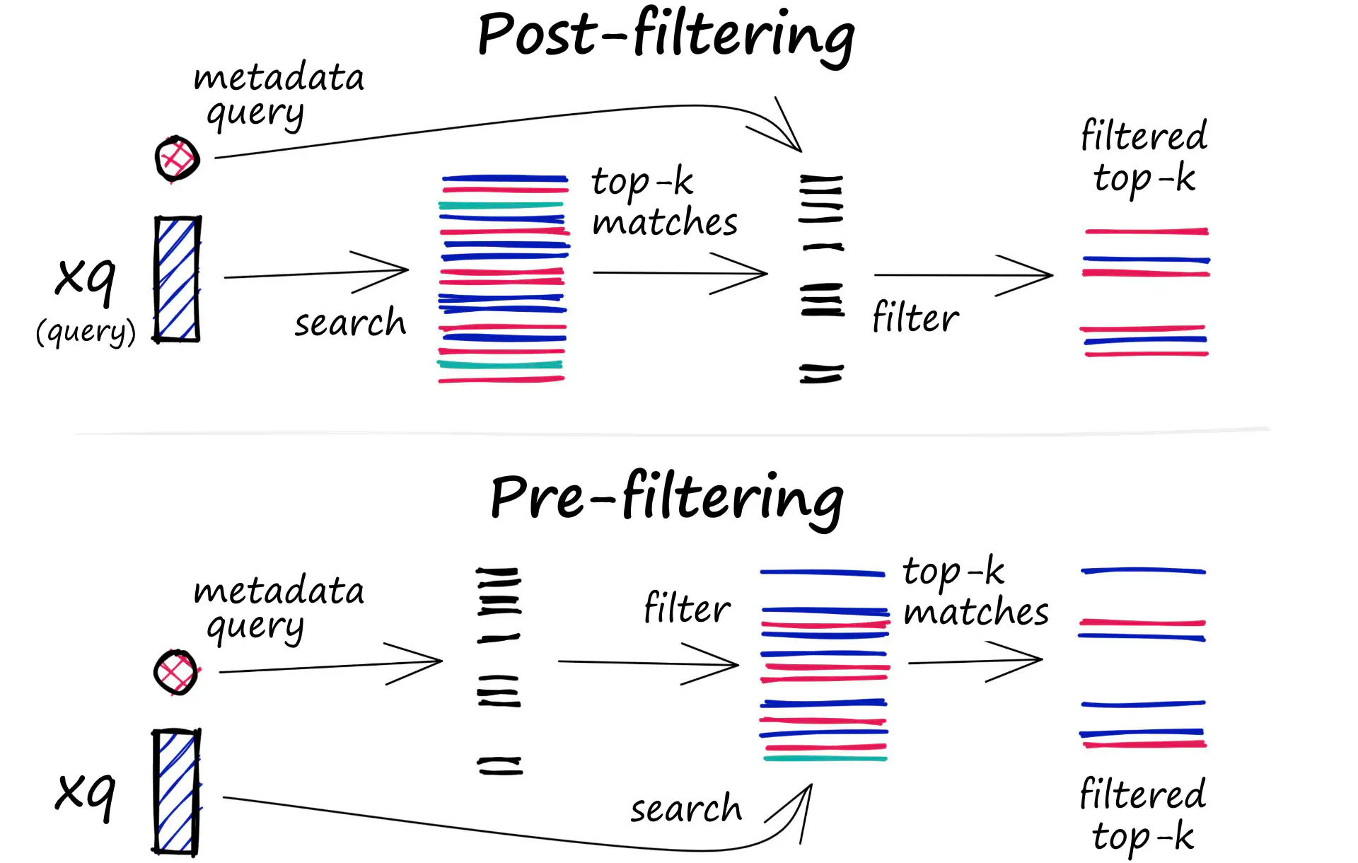
Post-Processing: Filtering

In addition to querying for similar vectors, vector databases can also filter the results based on a metadata query. To facilitate this, the vector database typically maintains two types of indexes: a vector index and a metadata index. Subsequently, it performs the metadata filtering either prior to or following the vector search:

• Pre-filter
  • The metadata filtering is conducted prior to the vector search. While this approach aids in reducing the search space, it can potentially result in the system disregarding pertinent results that do not align with the metadata filter criteria. Furthermore, excessive metadata filtering may slow down the query process due to the added computational overhead.
• Post-filter
  • The metadata filtering is conducted subsequent to the vector search. It assists in guaranteeing that all relevant results are taken into account. However, it may also introduce supplementary overhead and delay the query process, as irrelevant results must be filtered out post-search completion.

$\mathbf{Fig\ 7.}$ Pre-filtering v.s. Post-filtering (source: Pinecone)

Chroma

Chromais one of the most popular AI-native open-source vector databases. Chroma simplifies the development of LLM applications by making knowledge, facts, and skills easily pluggable for LLMs. Chroma enables users to:

• Store embeddings and their metadata;
• Embed documents and queries;
• Search embeddings;

$\mathbf{Fig\ 8.}$ LLM apps supported by Chroma (source: Chroma)

Chroma operates as follows:

1. Create a collection, which is similar to the tables in the relations database.
2. Chroma converts the text into the embeddings using sentence transformer (default: all-MiniLM-L6-v2).
3. Add text documents to the newly created collection with metadata and a unique ID. When your collection receives the text, it automatically converts it into embedding.
4. Query the collection by text or embedding to receive similar documents. You can also filter out results based on metadata.

and the following four core commands facilitate these operations:

# python can also run in-memory with no server running: chromadb.PersistentClient()

import chromadb
client = chromadb.HttpClient()
collection = client.create_collection("sample_collection")

# Add docs to the collection. Can also update and delete. Row-based API coming soon!
collection.add(
    documents=["This is document1", "This is document2"], # we embed for you, or bring your own
    metadatas=[{"source": "notion"}, {"source": "google-docs"}], # filter on arbitrary metadata!
    ids=["doc1", "doc2"], # must be unique for each doc 
)

results = collection.query(
    query_texts=["This is a query document"],
    n_results=2,
    # where={"metadata_field": "is_equal_to_this"}, # optional filter
    # where_document={"$contains":"search_string"}  # optional filter
) 

LangChain

LangChain is a framework designed to facilitate the development of applications driven by large language models (LLMs), streamlining the integration of LLMs into these applications. Much like the ODBC or JDBC drivers for databases, which obscure the complexities of SQL statement implementations, LangChain abstracts the intricacies of underlying LLMs by offering a straightforward and unified API.

Furthermore, LangChain is a powerful framework that seamlessly integrates with external tools to create a comprehensive ecosystem. It allows developers to effortlessly interchange models without requiring substantial modifications to the code.

Overall Flow

The following figure illustrates the overall pipeline of LangChain:

$\mathbf{Fig\ 9.}$ Overall flow of LangChain (source: Muhammad Waseem)

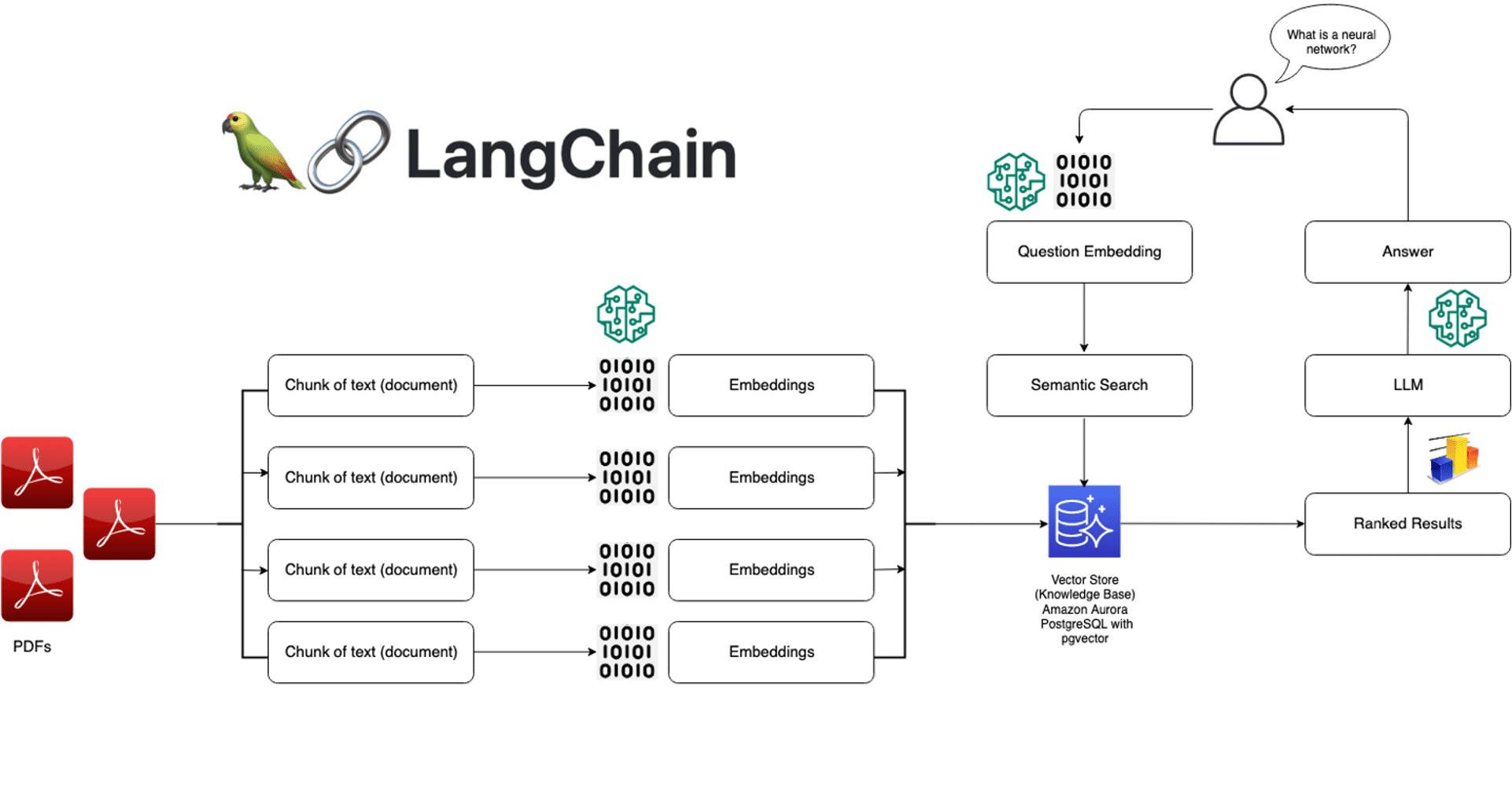
1. Data Sources
First, gather data from external sources such as PDFs, web pages, CSV files, and relational databases to construct the context for the LLM. LangChain effortlessly integrates with modules capable of accessing and retrieving data from these diverse sources.

# for PDF file we need to import PyPDFLoader from langchain framework
from langchain.document_loaders import PyPDFLoader
# for CSV file we need to import csv_loader
from langchain.document_loaders import csv_loader
# for Doc we need to import UnstructuredWordDocumentLoader
from langchain.document_loaders import UnstructuredWordDocumentLoader
# for Text document we need to import TextLoader
from langchain.document_loaders import TextLoader

import os # import os to set environment variable
os.environ['OPENAI_API_KEY'] = "apiKey" # Assign OpenAI API Key to environment variable  
loader = PyPDFLoader('filePath') # Init loader
documents = loader.load() # Load document 

2. Word Embeddings
The data retrieved from some of the external sources must be converted into vectors. This is done by passing the text to a word embedding model associated with the LLM.

from langchain.embeddings import OpenAIEmbeddings # Get embeddings model from Langchain framework. Other models are also possible.
embedding = OpenAIEmbeddings() # Define embedding

3. Vector DBs
The generated embeddings are stored in a vector database to facilitate similarity searches. LangChain simplifies the process of storing and retrieving vectors from various sources, including in-memory arrays and hosted vector databases such as Chroma and Pinecone.

# Embed and store the texts
from langchain.vectorstores import Chroma      
# Supplying a persist_directory will store the embeddings on disk
persist_directory = "myData" # e.g., we are saving data in myData folder in current application path
vectordb = Chroma.from_documents(documents=texts, embedding=embedding, persist_directory=persist_directory)
vectordb.persist() # save document locally
vectordb = None

4. LLMs
LangChain supports mainstream LLMs offered by OpenAI, Cohere, and AI21 and open source LLMs available on Hugging Face. It send prompt to LLM and retrieve response.

# Get the embedding and connect to VectorDB
embedding = OpenAIEmbeddings(model="text-embedding-ada-002",  chunk_size=1 )
vectordb = Chroma(persist_directory=persist_directory, embedding_function=embedding)

# Convert vector DB into retriever
retriever = vectordb.as_retriever()

# Load LLM, get an answer from LLM and send it back to the user 
llm = AzureChatOpenAI(deployment_name='gpt-35-turbo',  max_tokens=500)
qa_chain = RetrievalQA.from_chain_type(llm=llm, chain_type='stuff',retriever=retriever)
llm_response = qa_chain(query)
print(llm_response["result"])

Modules

The below figure represents the core of LangChain framework.

$\mathbf{Fig\ 10.}$ LangChain application architecture (source: Janakiram MSV)

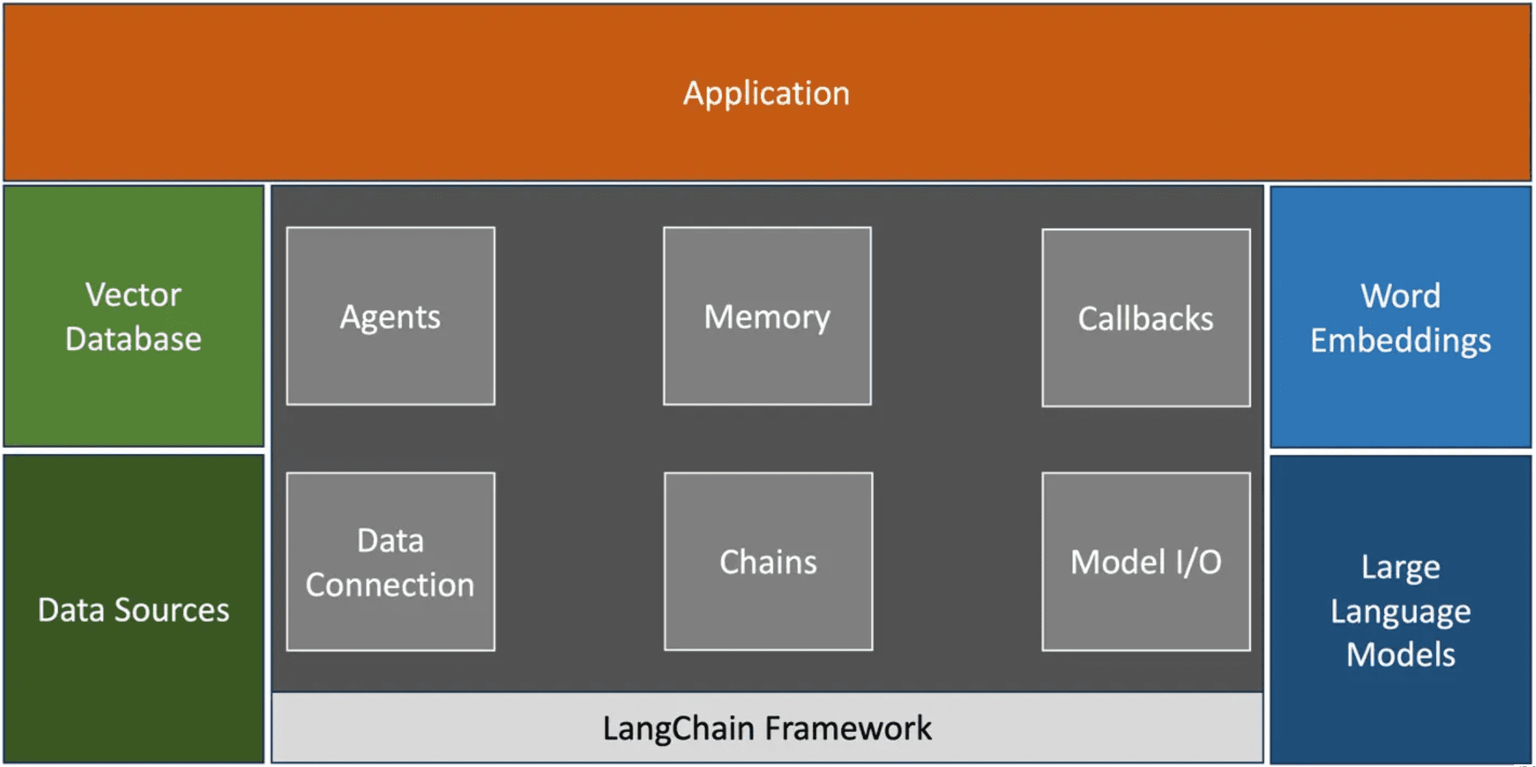
The applications at the top of the stack interact with one of the LangChain modules through the Python or JavaScript SDK. LangChain provides standard, extendable interfaces and external integrations for the following main components:

• Model I/O: the interaction with the LLM
  • It assists in creating effective prompts (prompt engineering), invoking the model API, and parsing the output
  • It abstracts the authentication, API parameters, and endpoint exposed by LLM providers
• Data connection: connection to the external documents
  • It deals with load external documents such as PDF, excels, etc., converting them into chunks for processing them into word embeddings in batches, storing the embeddings in a vector DB, and finally retrieving them through queries
• Chains: build efficient pipelines that leverage the building blocks and LLMs to get an expected response
  • It is possible to build highly complex chains that invoke the LLM multiple times, like recursion, to achieve an outcome
    • For example, a chain may include a prompt to summarize a document and then perform a sentiment analysis on the same
• Memory: enables coherent conversation
  • LLMs are stateless but need context to respond accurately. The memory module makes it easy to add both short-term and long-term memory to models
    • Short-term memory maintains the history of a conversation through a simple mechanism; message history can be persisted to external sources such as Redis, representing long-term memory
• Callbacks: hook developers into the various stages of an LLM application
  • This is useful for logging, monitoring, streaming, and other tasks
  • It is possible to write custom callback handlers that are invoked when a specific event takes place within the pipeline
• Agents
  • LLMs are capable of reasoning and acting, called the ReAct prompting technique; the agents simplify crafting ReAct prompts that use the LLM to distill the prompt into a plan of action
    • The basic idea behind agents is to use an LLM to select a set of actions
    • A sequence of actions is hard-coded in chains (in code), and LLM is used as a reasoning engine in agents to determine which actions to take and in what order

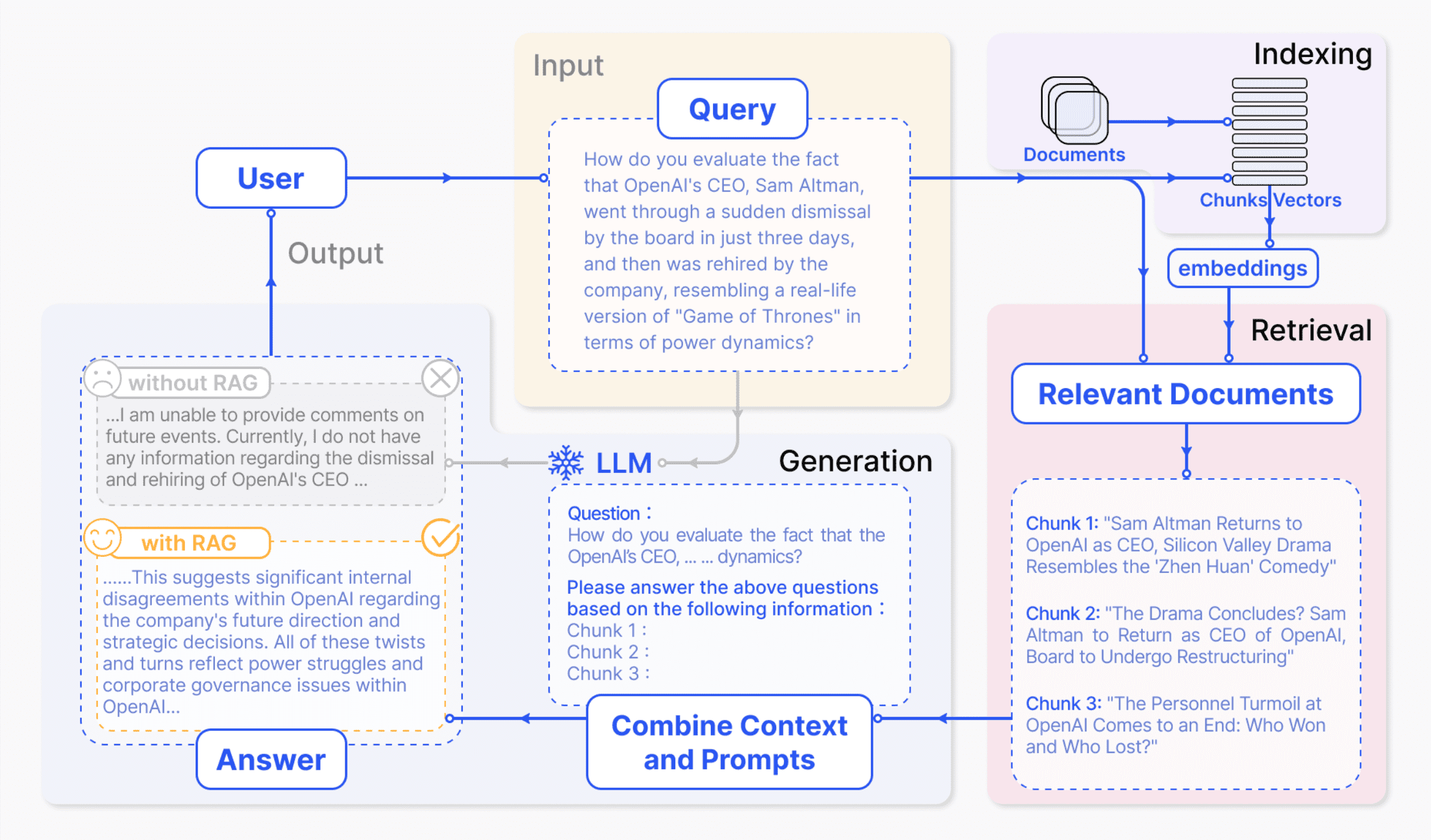
Retrieval-Augmented Generation (RAG)

LLMs possess the capacity to deliberate on diverse subjects, but their knowledge is confined to publicly available data up to a particular training point in time. To build AI applications capable of reasoning about private data or post-cutoff date data, augmenting the model’s knowledge becomes imperative. This entails retrieving pertinent information and seamlessly incorporating it into the model prompt, which is known as Retrieval Augmented Generation (RAG). A typical application of RAG is illustrated in the following figure:

$\mathbf{Fig\ 11.}$ LangChain application architecture (source: Gao et al. 2023)

Architecture

A typical RAG application comprises two main components:

• Indexing
  • A pipeline for ingesting data from a source and indexing it, usually performed offline
• Retrieval & Generation
  • The actual RAG chain, which processes the user query in real time, retrieves the relevant data from the index, and then passes it to the model

Depending on the literature, retrieval and generation are sometimes described as separate components.

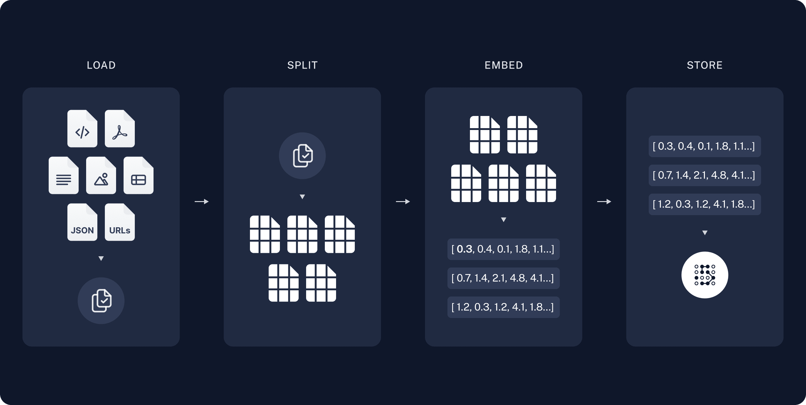
Indexing

To address the context limitations inherent in language models, text is divided into smaller, more manageable chunks. These chunks are then encoded into vector representations via an embedding model and stored in a vector database. This process is essential for facilitating efficient similarity searches in the subsequent retrieval phase.

$\mathbf{Fig\ 12.}$ RAG Indexing (source: LangChain)

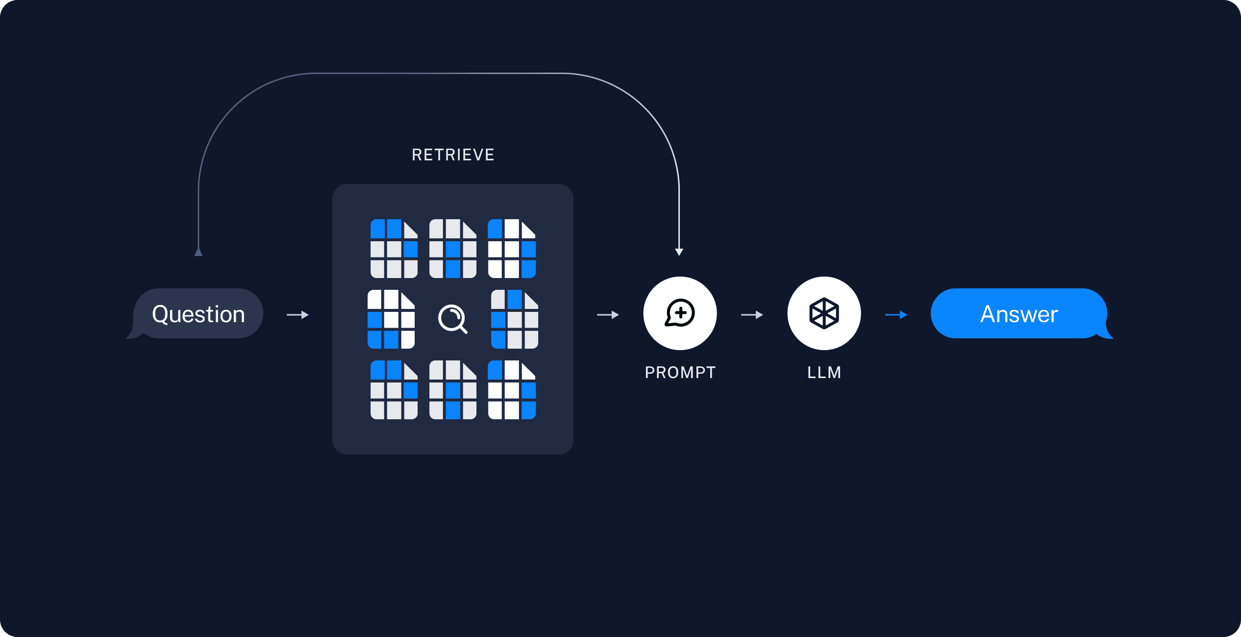
Retrieval

Upon receipt of a user query, the RAG system employs the same encoding model used during the indexing phase to transform the query into a vector representation. It then calculates similarity scores between the query vector and the vectors of chunks within the indexed corpus. The system prioritizes and retrieves the top $K$ chunks that exhibit the highest similarity to the query. These chunks are subsequently utilized as the expanded context in the prompt.

Generate

The posed query and selected documents are synthesized into a coherent prompt, which a LLM is tasked with using to formulate a response. The model’s approach to answering may vary based on task-specific criteria, allowing it to either draw upon its inherent parametric knowledge or limit its responses to the information contained within the provided documents. In cases of ongoing dialogues, any existing conversational history can be integrated into the prompt, enabling the model to engage iengage effectively in multi-turn dialogue interactions.

$\mathbf{Fig\ 13.}$ RAG Retrieval and Generation (source: LangChain)

References

[1] Roie Schwaber-Cohen, Pinecone, “What is a Vector Database & How Does it Work? Use Cases + Examples”, 2023
[2] Frank Liu, Director of Operations & ML Architect at Zilliz, “What is a Vector Database?”, 2024
[3] Pavan Belagatti, “WTF Is a Vector Database: A Beginner’s Guide!”, 2023
[4] Dominik Polzer, “All You Need to Know about Vector Databases and How to Use Them to Augment Your LLM Apps” Towards Data Science 2023
[5] Chris McCormick, “Product Quantizers for k-NN Tutorial Part 1”, 2017
[6] Vyacheslav Efimov, “Similarity Search, Part 4: Hierarchical Navigable Small World (HNSW)”, Towards Data Science, 2023
[7] Chroma Docs
[8] datacamp, Chroma DB Tutorial: A Step-By-Step Guide
[9] Janakiram MSV, “A brief guide to LangChain for software developers”, InfoWorld
[10] Muhammad Waseem, “Step by step guide to create personalized AI with ChatGPT by using LangChain”, InterSystems Developer Community
[11] LangChain Document
[12] Gao et al., “Retrieval-Augmented Generation for Large Language Models: A Survey”, arXiv:2312.10997