[DL] Dropout

In this post, we will discuss about one technique called dropout to get neural networks to generalize better.

Motivation: Ensembles

In usual, neural networks have many trainable parameters, so that it often suffers from high variance. And since there are usually many more ways to be wrong than to be right, once models are trained well with respect to the given dataset they may disagree on the wrong answer, even they will agree on the different right answers due to high variance.

Ensembles combine multiple hypotheses to form a (hopefully) better hypothesis. There are various ways for ensemble learning, such as Bayesian model averaging, etc. But in this post, we will take bootstrap aggregating (bagging) ensemble for an example.

Example: Bootstrap Aggregating Ensembles

Let \(\mathcal{D} = \{ (x_i, y_i) \}\) be a given dataset. Our goal is to train multiple independent models that are trained on different independent dataset. One simple approach is to split a huge dataset into some number of non-overlapping parts. However such an approach is somewhat wasteful as we’re essentially training each model in a much smaller amounts of datasets.

So, we will resample the given dataset by picking $N$ datapoints randomly with replacement. In other words, we will obtain independently sampled datasets

\[\begin{aligned} D_j = \{ (x_{i_{j, 1}}, y_{i_{j, 1}}), (x_{i_{j, 2}}, y_{i_{j, 2}}), \cdots, (x_{i_{j, N}}, y_{i_{j, N}}) \} \end{aligned}\]

where $i_{j, k}$s are randomly selected in \(\{ 1, \cdots, N \}\) by allowing for repeatition. These datasets are called bootstrapped sets:

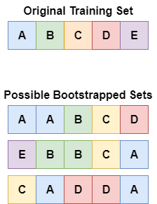
$\mathbf{Fig\ 1.}$ Bootstrap set generation (source: [5])

Then, we can obtain separately trained models $p_{\theta_j} (y | x)$ for $j = 1, \dots, M$. And we finalize our prediction by averaging the predicted probabilities $p( y | x ) = \frac{1}{M} \sum_{j=1}^M p_{\theta_j} (y | x)$, or majority voting.

Example: Snapshot Ensemble

In case of deep learning, we often getmuch of the same benefit without resampling in practice, as there is already a lot of randomness in training of neural network.

• Random initialization
  
• SGD
  
• Data shuffling
  

Snapshot Ensembles [6] is a representative example of this. It simply trains different models, but on the same dataset $\mathcal{D}$. The idea is to save out parameter snapshots over the SGD training procedure, and use each snapshot as a model in the ensemble:

1. Initialize the model
2. Train for a short period (e.g. 50 epochs per 300 epochs) with a cyclic lr scheduler
3. Take a snapshot
4. Continue training with a "new" cyclic lr scheduler for another short period
5. Take a snapshot
6. Repeat
7. Ensemble the snapshots (by averaging predictions)

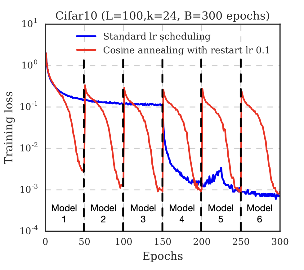
$\mathbf{Fig\ 2.}$ Snapshot Ensembles [6]

The following left figure shows the procedure of finding global optimum by descending through gradient with standard SGD optimization, and snapshot ensemble:

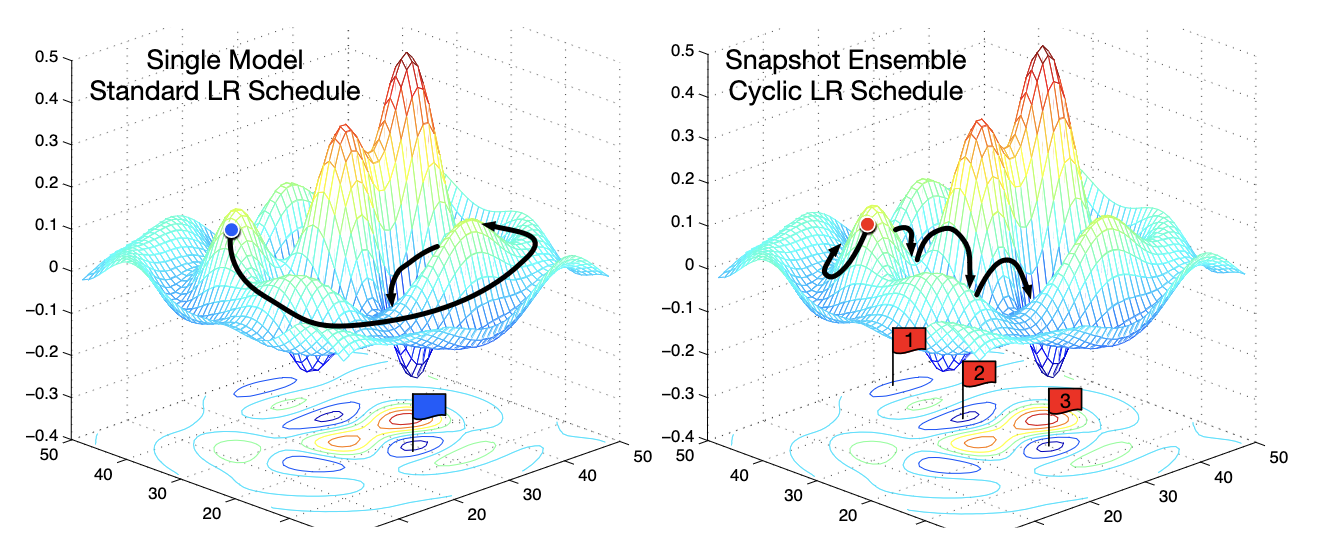
$\mathbf{Fig\ 3.}$ SGD optimization v.s. Snapshot Ensembles [6]

In snapshot ensembles, the different models undergo the convergence to multiple local minima. Each time the model converges, we take a snapshot of model, and escape the local minimum to restart the optimization.

Although the original paper aggregated snapshots by averaging the predictions, ensembles with other ways such as majority voting and parameter averaging is still available.

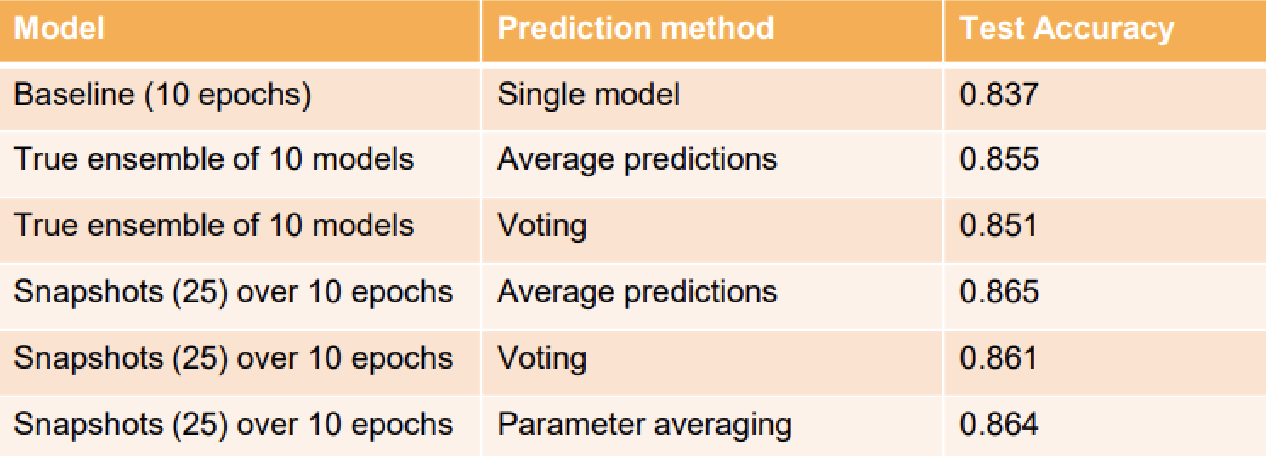
$\mathbf{Fig\ 4.}$ Ensembles comparisons (source: [4])

Dropout

Ensembles of different models is also a powerful way to regularize. Because, even if a model tries to overfit, other models may not. And the bigger the ensemble is, the better it performs usually even it is much expensive. How can we obtain many different neural networks efficiently?

Dropout achieves this only with a single neural network by randomly clamping on/off hidden units with some probability $p$. (This can be considered as a random sampling of network architecture.)

$\mathbf{Fig\ 5.}$ Dropout (source: [1])

A neural network with $n$ nodes can be seen as a huge collection of $2^n$ possible neural networks if dropout is applied. So training a neural network with dropout can be seen as training a collection of $2^n$ thinned networks with extensive weight sharing, i.e. ensemble effect.

Also, dropout forces the network to have a redundant representation, so that it less sensitive and dependent to the particular features and can’t rely on the combination (or interaction) of them, i.e. prevents co-adaptation of features:

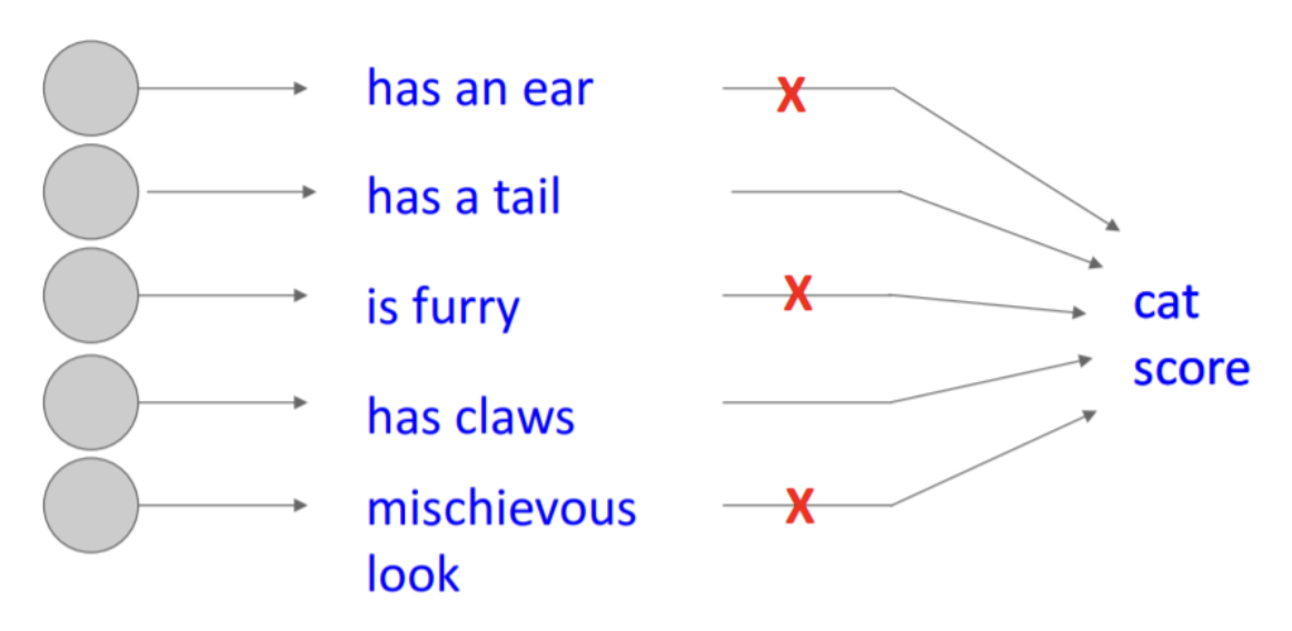
$\mathbf{Fig\ 6.}$ Dropout forces the network to have a redundant feature

For example in the figure above, envision the training dataset that has the pictures of cats with a tail sticking out only. Then, without dropout, since the feature “has a tail” is always present the model can be trained to classify an object as a cat only if an object has a tail.

But it is also a cat!

Hence, dropout makes the neural networks more robust and prevents the overfitting problem (this can be also impart due to reduction of the number of parameters). Also a lot of literatures reports that it has smaller generalization error on a wide variety of tasks.

At train time

For each training case in a mini-batch, we sample a thinned network by dropping out units. Forward and backpropagation for that training case are done only on this thinned network. The gradients for each parameter are averaged over the training cases in each mini-batch.

For example, consider a fully-connected network’s operation

\[\begin{aligned} z_i^{(\ell + 1)} &= \mathbf{W}_i^{(\ell + 1)} \mathbf{y}^\ell + b_i^{(\ell + 1)} \\ y_i^{(\ell + 1)} &= f(z_i^{(\ell + 1)}) \end{aligned}\]

With dropout of rate $p$, it becomes

\[\begin{aligned} m_j^{(\ell)} &\sim \text{Bernoulli}(p) \\ \widehat{\mathbf{y}}^{(\ell)} &= \mathbf{m}^{(\ell)} \cdot \mathbf{y}^{(\ell)} \\ z_i^{(\ell + 1)} &= \mathbf{W}_i^{(\ell + 1)} \widehat{\mathbf{y}}^\ell + b_i^{(\ell + 1)} \\ y_i^{(\ell + 1)} &= f(z_i^{(\ell + 1)}) \end{aligned}\]

At test time

We want to combine all possible models and use the whole network at test time like regular resemble. But, we should multiply the outgoing weights of each unit by $1 - p$. (Or, it is also mathematically equivalent to multiply $\frac{1}{1 - p}$ to activations at training time)

This ensures that for any hidden unit, the expected output under the distribution used to drop units at training time is the same as the actual output at test time. And it corresponds to taking an average of predictionsc of different models to finalize the prediction in ensemble learning.

Reference

[1] Kevin P. Murphy, Probabilistic Machine Learning: An introduction, MIT Press 2022.
[2] CS231n: Convolutional Neural Networks for Visual Recognition
[3] N. Srivastava et al., Dropout: A Simple Way to Prevent Neural Networks from Overfitting, Journal of Machine Learning Research, pp. 1929–1958, 2014.
[4] UC Berkeley CS182: Deep Learning, Lecture 9 by Sergey Levine
[5] Wikipedia, Ensemble learning
[6] Huang, Gao, et al. “Snapshot ensembles: Train 1, get m for free.” arXiv preprint arXiv:1704.00109 (2017).