[DL] Recurrent Neural Network

Pipeline of RNN (source)

Motivation: Sequence Modeling

Sequence modeling is prevalent in many data like language, video, etc. Main characteristic of sequential data is variable input & output length. Also, there exists temporal dependency in the data.

Hence for language model, it would be beneficial to predict the next word from the information of past words:

\[\begin{aligned} p(\mathbf{x}) = \prod_{i=1}^n p(x_i | x_1, \cdots, x_{i-1}) = \prod_{i=1}^n p(x_i | \mathbf{x}_{< i}) \end{aligned}\]

Let’s try to make a neural language model using an MLP. This MLP is shared across the time steps:

The problem is that what has happened in the past is not considered in the future prediction. We can’t provide both “I” and “love” as input at the second timestep because MLP cannot deal with variable input length. So, it is memory-less.

So, if we can make the update of the hidden layer to be dependent not only on the input but on the previous hidden state, the current prediction will be aware of the past. Then, we can connect MLP as follows:

Here, standard update of MLP hidden is \(\mathbf{h}_t = \text{activation}(\mathbf{W} \mathbf{x}_t + b)\). By storing $\mathbf{h}_{t-1}$, we can modify this to \(\mathbf{h}_t = \text{activation}(\mathbf{Wx}_t + \mathbf{Vh}_{t-1 \to t} + \mathbf{b})\)

This, however, requires storing weights $\mathbf{W}$ and $\mathbf{Vh}_{t-1 \to t}$ for an undertermined length.

Recurrent Neural Network (RNN)

The solution is temporal weight sharing.

RNN architecture (source: Andrej Karpathy)

Let

• $N$: mini-batch size
  
• $D$: input dim
  
• $H$: hidden layer dim
  
• $K$: number of output classes
  

Then,

\[\begin{aligned} &\mathbf{h}_t = \sigma(\mathbf{W}_{\text{xh}} \mathbf{x}_t + \mathbf{W}_{\text{hh}} \mathbf{h}_{t-1} + \mathbf{b}) \\ &\mathbf{y}_t = f(\mathbf{W}_{\text{hy}} \mathbf{h}_t + \mathbf{c}) \end{aligned}\]

where

• $\mathbf{x}_t \in \mathbb{R}^{D \times N}$
• $\mathbf{W}_{\text{xh}} \in \mathbb{R}^{H \times D}$
• $\mathbf{h}_t \in \mathbb{R}^{H \times N}$
• $\mathbf{W}_{\text{hh}} \in \mathbb{R}^{H \times H}$
• $\mathbf{b} \in \mathbb{R}^{H}$
• $\mathbf{c} \in \mathbb{R}^{H}$
• $\mathbf{y}_t \in \mathbb{R}^{K \times N}$

Cost Function

RNN predicts one of the word in the token collection at each timestep, thus we can use the cost functions that are used in the classification problem. For instance, maximum likelihood estimation of a sequence through NLL loss is one possible option. The likelihood of $\mathbf{x}$ is

\[\begin{aligned} p_{\theta} (\mathbf{x}) = p_{\theta} (x_1, \cdots, x_T) = \prod_{t=1}^T p_{\theta} (x_t | \mathbf{x}_{< t}) \end{aligned}\]

With multiple training sequences \(D = \{ \mathbf{x}^{(1)}, \cdots, \mathbf{x}^{(N)} \}\), we minimize negative log-likelihood (NLL):

\[\begin{aligned} L(\theta; D) = - \sum_{n=1}^N \sum_{t=1}^{T_n} \text{log } p_{\theta} (x_{t}^{(n)} | \mathbf{x}_{< t}^{(n)}) \end{aligned}\]

Here, $\mathbf{x_{< t}}$ can be modeled as RNN’s hidden state \(\mathbf{h_{t-1}} = \text{RNN}_{\theta} (\mathbf{h_{t-2}}, x_{t-1})\). That is, $\mathbf{h_{t-1}}$ can be seen a learned representation or a compression of $\mathbf{x_{< t}}$

\[\begin{align*} p_{\theta} (x_{t} = k | \mathbf{x}_{< t} = \mathbf{h}_{t-1}) = \text{softmax} (\mathbf{w}_k \mathbf{h}_{t-1}) = \frac {\text{exp}(\mathbf{w}_k \mathbf{h}_{t-1})} {\sum_j \text{exp}(\mathbf{w}_j \mathbf{h}_{t-1})} \end{align*}\]

where $k$ can be the index of a word in the vocabulary in language modeling. Then, we can apply automatic differentiation to compute the gradient. Recall that, for $k$-class classification, minimizing NLL is the same as minimizing cross entropy.

\[\begin{aligned} \text{CE}(q, p) &= - \sum_{j=1}^K q(x = j) \cdot \text{log } p(x = j) \\ &= -\text{log } p(x = k) \\ &= \text{NLL}(p, k) \end{aligned}\]

Teaching Forcing

We use the predicted value to the next input in RNN, but the predicted value might be incorrect and it may problematic since the error can be compounded. Instead, during training, we just insert the ground truth label to the RNN at next timestep, regardless of the previous prediction.

And this techinqiue is referred to as teaching forcing.

Unfortunately, it can sometimes work poorly at test time, since the model has only ever been trained on correct inputs. The network always saw true sequences as inputs in the training time but at test-time it gets as input its own (potentially incorrect) predictions. This is called distributional shift, because the input distribution shifts from true strings (at training) to synthetic strings (at test time).

Thus, it may not learned how to deal with input sequence generated from the previous step, $\widehat{x}_{1:t-1}$, that deviates from what it saw in training. To deal with this, we usually do not use teaching forcing completely: use teaching forcing, but at random time steps, feeds in samples from the model instead of ground truth. And it is called scheduled sampling.

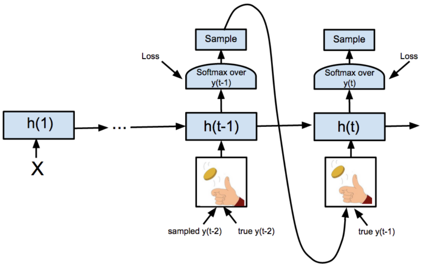
Scheduled sampling (source: S. Bengio et al. 2015)

The authors recommend to gradually increase the probability of feeding the predicted output as an input to realize this aspect. In other words, at the beginning of training, we usually mostly feed in ground truth tokens as input, since model predictions are mostly nonsense. And then at the end of training, we mostly feed in the model’s own predictions, to mitigate distribution shift in the test-time.

Backpropagation Through Time (BPTT)

So, how can we compute the gradient of an RNN? Due to the temporal parameter sharing, this may not seem obvious.

We can explicitly draw the computation graph of an RNN by unrolling the networks along the time axis. We can then simply apply the standard backpropagation on this graph. (Of course, we don’t have to unroll during test time.) This is called backpropagation through time (BPTT).

But, what if we have a very long sequence, for example $T = \text{10K}$? BPTT shows the problem such as

• memory
  
• vanishing gradients
  

So, we usually truncate the sum to the most recent $K$ terms, and it is called truncated BPTT (T-BPTT).

Truncated BPTT

Truncated BPTT splits the full sequence into several segments.

We just train the one segment at once to reduce the memory load of GPU. The typical way of training is carrying over the hidden state across segment updates during training:

Forward Pass
For each segment, we set the initial hidden state of a segment to the last hidden state of the previous segment, so information can be propagated longer than a segment.

Backpropagation
Compute the gradient by backpropagation only within the current segment. As we have to store just only the hidden states of the current segment, small memory resources are needed in contrast to normal BPTT.

However, the limitation of it is straight-forward: Inter-segment long-term dependency cannot be learned. Also, the cells of the previous segment cannot updated with respect to the current error.

Bi-Directional RNN

The basic RNN can only use the information of the past. However, what if the full sequence is given at inference time unlike the word prediction? In bi-directional RNN, forward and backward hidden states are concatenated to provide representations to the output layer. To do this, we create two RNNs, one which recursively computes hidden states in the forwards direction, and one which recursively computes hidden states in the backwards direction.

Precisely,

\[\begin{aligned} &\mathbf{h}_t^{\leftarrow} = \sigma( \mathbf{W}_{\text{xh}}^{\leftarrow} \mathbf{x}_t + \mathbf{W}_{\text{hh}}^{\leftarrow} \mathbf{h}_{t-1}^{\leftarrow} + \mathbf{b}_{\text{h}}^{\leftarrow} ) \\ &\mathbf{h}_t^{\rightarrow} = \sigma( \mathbf{W}_{\text{xh}}^{\rightarrow} \mathbf{x}_t + \mathbf{W}_{\text{hh}}^{\rightarrow} \mathbf{h}_{t+1}^{\rightarrow} + \mathbf{b}_{\text{h}}^{\rightarrow} ) \\ \end{aligned}\]

Then, we define the representation of the state at time $t$, $\mathbf{h}_t$

\[\begin{align*} \mathbf{h}_t = [\mathbf{h}_t^{\leftarrow}, \mathbf{h}_t^{\rightarrow}] \end{align*}\]

and generate the output at time $t$ with this hidden state $\mathbf{h}_t$.

Deep RNN

Like Deep Nerual Network, we can create more expressive models by stacking multiple hidden layers on top of each other. In Deep RNN, each hidden layer has different parameters but shared temporally. (Note that it works vertically.)

Precisely,

\[\begin{align*} \mathbf{h}_t^l = \sigma_l (\mathbf{W}_{\text{xh}}^l \mathbf{h}_t^{l - 1} + \mathbf{W}_{\text{hh}}^l \mathbf{h}_{t-1}^l + \mathbf{b}_{\text{h}}^l) \end{align*}\]

Then, the output is given by

\[\begin{align*} \mathbf{o}_t = \mathbf{W}_{\text{ho}} \mathbf{h}_t^L + \mathbf{b}_{\text{o}} \end{align*}\]

Difficulties in Training RNNs

Some optimization helper tools like weight intialization, faster optimizers, dropout, … etc. also works well for RNN. But, we usually DO NOT USE RELU.

Because, its unboundedness can facilitate explosion in forward-propagation due to sharing of the same weights. Similarly, the gradient explodes more easily. (But in this case, we can use gradient clipping).

Also, batch normalization is not very useful in RNNs.

Reference

[1] Kevin P. Murphy, Probabilistic Machine Learning: An introduction, MIT Press 2022.
[2] UC Berkeley CS182: Deep Learning, Lecture 10 by Sergey Levine
[3] Is it normal to use batch normalization in RNN & LSTM?