[DL] LSTM & GRU

Pipeline of LSTM (source)

Gradient Vanishing & Explosion of RNN

In the previous post, we saw the neural network for sequences, RNN, which updates its parameter recurrently for each timestep. However, nowadays, we do not use this original RNN due to gradient vanishing & explosion problem. It is because we multiply the hidden state by the weight matrix continuously at each time step (so does gradient). If we denote the $i$-th loss term of RNN, then the gradient of the loss with respect to an arbitrary hidden state $\boldsymbol{h}^{(j)}$

\[\begin{aligned} \frac{\partial J^{(i)}(\theta)}{\partial \boldsymbol{h}^{(j)}}=\frac{\partial J^{(i)}(\theta)}{\partial \boldsymbol{h}^{(i)}} \prod_{j<t \leq i} \frac{\partial \boldsymbol{h}^{(t)}}{\partial \boldsymbol{h}^{(t-1)}} \end{aligned}\]

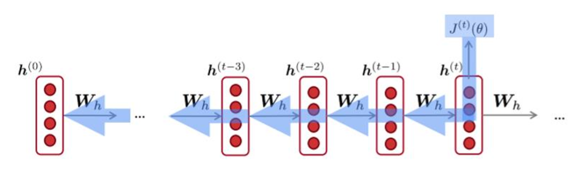
We can simply use gradient clipping for gradient explosion, but in practice vanilla RNNs fail to remember inputs from long in the past due to vanishing gradient problem. To solve this, we usually use RNN with modified architecture, LSTM and GRU, which significantly improves the stability of model. It updates the hidden state in an additive way, not a multiplication, similar to a residual net.

---

LSTM

The basic idea of gated RNN is, we want $\frac{d \mathbf{h}^{(t)}}{d \mathbf{h}^{(t-1)}} \approx 1$ if we choose to remember $\mathbf{h}^{(t-1)}$ in the next time step, so that we propagate the memory by preventing vanishing gradient. So, we may construct a litte neural circuit that decides whether to remember or overwrite:

• if “remembering”, maintain the previous state
• if “forgetting”, replace it by another vector, based on the current input

Hence, we add another state of RNN, cell state \(\mathbf{C}_t\) that acts as a long-term memory. And we set the dynamic of RNN to be \(\frac{d \mathbf{h}^{(t)}}{d \mathbf{h}^{(t-1)}} = \mathbf{F}_t \in [0, 1]\) so it can regularize the extent of memory itself. And the generalization of this idea is LSTM (Long Short Term Memory).

It determines to forget the past memory \(\mathbf{C}_{t-1}\) and memorize new memory \(\widetilde{\mathbf{C}}_t\). And on the top of the current memory \(\mathbf{C}_{t}\), constructs new abstraction (hidden state) \(\mathbf{H}_t\). All pathes for forget, memory, and proposal are determined by the forget, input, and output gates \(\mathbf{F}_t\), \(\mathbf{I}_t\), and \(\mathbf{O}_t\) respectively, which are generated by input data \(\mathbf{X}_t\) and the previous hidden state \(\mathbf{H}_{t-1}\).

Here, the cell state \(\mathbf{C}_{t}\) with additive update changes very little step to step, in contrast to the hidden state \(\mathbf{H}_{t}\) which essentially overwritten by the non-linear operation of \(\mathbf{C}_{t}\) changes all the time. Thus \(\mathbf{C}_{t-1}\) is considered as long-term memory, and \(\mathbf{H}_{t}\) is considered as short-term memory.

In summary,

• Memory update \(\mathbf{C}_t = \mathbf{F}_t \odot \mathbf{C}_{t-1} + \mathbf{I}_t \odot \mathbf{\widetilde{C}}_t\)

• Next hidden state \(\mathbf{H}_t = \mathbf{O}_t \odot \text{tanh }(\mathbf{C}_t)\)

• Candidate cell state \(\widetilde{\mathbf{C}}_t = \text{tanh} (\mathbf{X}_t \mathbf{W}_{\text{xc}} + \mathbf{H}_{t-1} \mathbf{W}_{\text{hc}} + \mathbf{b}_{\text{c}})\)

• Input / Forget / Output Gates

\[\begin{aligned} \mathbf{I_t} &= \sigma (\mathbf{X}_t \mathbf{W}_{\text{xi}} + \mathbf{H}_{t-1} \mathbf{W}_{\text{hi}} + \mathbf{b}_{\text{i}}) \\ \mathbf{F_t} &= \sigma (\mathbf{X}_t \mathbf{W}_{\text{xf}} + \mathbf{H}_{t-1} \mathbf{W}_{\text{hf}} + \mathbf{b}_{\text{f}}) \\ \mathbf{O_t} &= \sigma (\mathbf{X}_t \mathbf{W}_{\text{xo}} + \mathbf{H}_{t-1} \mathbf{W}_{\text{ho}} + \mathbf{b}_{\text{o}}) \\ \end{aligned}\]

$\mathbf{Fig\ 1.}$ LSTM architecture (source: [1])

These formulations seem to be a little bit arbitrary, but it ends up working well in practice and much better than vanilla RNN.

GRU

We see that the internal operation of LSTM is much complicate than vanilla RNN, and one may wonder some operation is indeed necessary. Unlike LSTM, there is no separation of memory and hidden state in GRU (Gated Recurrent Unit), so it has better space complexity than LSTM. Also, GRU has only two gates:

• Reset / Update Gates
  

\[\begin{aligned} \mathbf{R_t} &= \sigma (\mathbf{X}_t \mathbf{W}_{\text{xr}} + \mathbf{H}_{t-1} \mathbf{W}_{\text{hr}} + \mathbf{b}_{\text{r}}) \\ \mathbf{Z_t} &= \sigma (\mathbf{X}_t \mathbf{W}_{\text{xz}} + \mathbf{H}_{t-1} \mathbf{W}_{\text{hz}} + \mathbf{b}_{\text{z}}) \end{aligned}\]

• Candidate next state computation: \(\mathbf{\widetilde{H}}_t = \text{tanh} (\mathbf{X_t} \mathbf{W}_{\text{xh}} + (\mathbf{R}_t \odot \mathbf{H}_{t-1}) \mathbf{W}_{\text{hh}} + \mathbf{b}_{\text{h}})\)

• State update: $\mathbf{H_t} = \mathbf{Z_t} \odot \mathbf{H_{t-1}} + (1 - \mathbf{Z_t}) \odot \mathbf{\widetilde{H}}_t$

$\mathbf{Fig\ 2.}$ GRU architecture (source: [1])

GRU v.s. LSTM

LSTM works better in general. But, for some problems, GRU provides similar performance as LSTM but with lower computation & space complexity.

RNN v.s. LSTM

In practice, vanilla RNN almost never work.

• Updating memory
  
  • RNN: updated_memory = nonlinear (old_memory + new_input)
  • LSTM: updated_memory = forget_gate $\odot$ old_memory + input_gate $\odot$ new_input
• Output (Hidden) states
  
  • RNN: output_states = updated_memory
  • LSTM: output_states = output_gate $\odot$ tanh(update_memory)
    

In a nutshell, the main differences between them are:

1. State update rule
2. Existence of gates
3. Separation of memory and output states

Inductive Biases of Gated RNNs

• Memorize (Not forgetting)
  

• Select what to memorize (Skippping inputs)
  

• Forget (Resetting memory)
  

• Vanilla RNNs need to learn these functions without much guidance
  $\to$ More explicit inductive bias applied to the architecture can be helpful!

Reference

[1] Kevin P. Murphy, Probabilistic Machine Learning: An introduction, MIT Press 2022.
[2] UC Berkeley CS182: Deep Learning, Lecture 10 by Sergey Levine