[DL] Seq2Seq

Sequence-to-sequence (Seq2seq) is referred to as a family of machine learning approaches for NLP, including applications in language translation, image captioning, and text summarization. As the name implies, it turns one sequence input into another sequence output. For example, translation to English from Korean.

Mathematically, the objective of seq2seq problem is to learn a function $f_\theta: \mathbb{R}^{TD} \to \mathbb{R}^{T^\prime D^\prime}$ where $T$ and $T^\prime$ are length of input and output, respectively.

Seq2seq model

To my knowledge, seq2seq indicates two different concepts. Many literatures also call the model proposed by [3] as a Seq2Seq model.

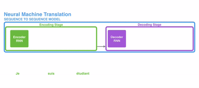
$\mathbf{Fig\ 1.}$ Seq2Seq model (source)

Seq2Seq model is a combination of Encoder RNN and Decoder RNN. Encoder RNN encodes the source sequence using a RNN, and the last hidden state of the encdoer RNN is used to initialize the decoder RNN. And it usually makes predictions at every step of the decoder. Hence, the decoder is a conditional language model:

\[\begin{aligned} p(y_1, y_2, \dots, y_{T^\prime} | \mathbf{x} = (x_1, x_2, \dots, x_T)) &= \prod_{t=1}^{T^\prime} p(y_t | y{<t}, \color{red}{\mathbf{x}}) \\ \end{aligned}\]

and as usual in RNN, the past inputs and outputs are abstracted into hidden state $\mathbf{h}$:

\[\begin{aligned} p(y_1, y_2, \dots, y_{T^\prime} | \mathbf{x} = (x_1, x_2, \dots, x_T)) &= \prod_{t=1}^{T^\prime} p(y_t | h_t^y, \color{red}{\mathbf{h}_T^{\mathbf{x}}}) \\ \end{aligned}\]

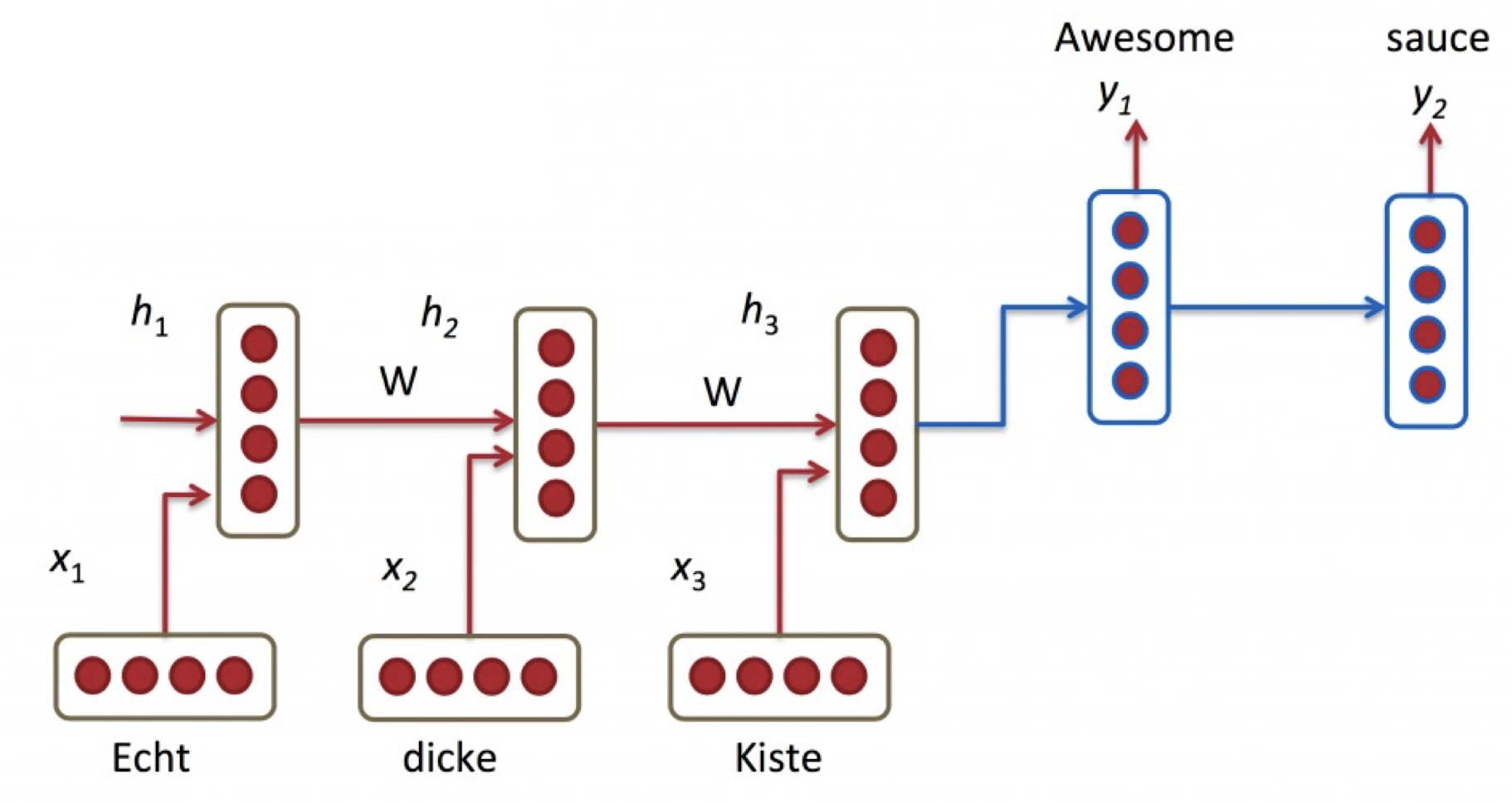
$\mathbf{Fig\ 2.}$ The input sequence is summarized (encoded) to hidden state of encoder

For instance, this structure can be employed for neural machine translation (NMT), as [3]:

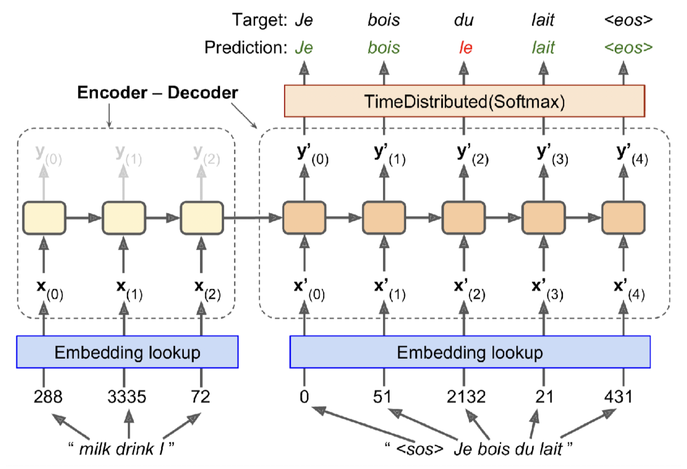
$\mathbf{Fig\ 3.}$ Seq2Seq model of neural machine translation

Decoding: Beam Search

The most intuitive way to generate a sequence from RNN is greedy decoding: to select a token that maximizes the probability for each timestep, i.e. \(\widehat{y}_t = \underset{y}{\text{argmax }} p(y_t = y \mid \mathbf{y}_{1:t-1}, \mathbf{x})\) as a classification task. And we repeat this until $y_t$ meet token.

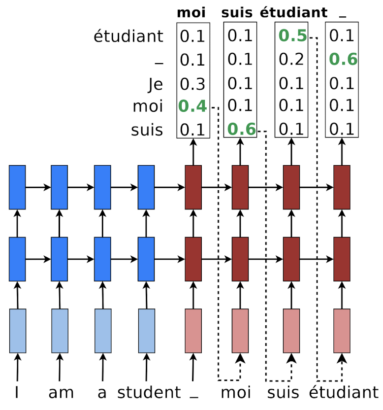
$\mathbf{Fig\ 4.}$ Greedy decoding (source: [1])

Unfortunately, greedy decoding will not always lead to the answer. For example, consider the following example. What if the second probable token generates outputs with much higher probability?

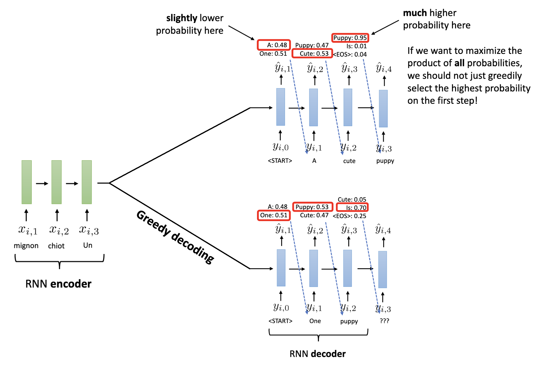
$\mathbf{Fig\ 5.}$ Counterexample of greedy decoding (source: [2])

In other words, as the locally optimal token at timestep $t$ might not be on the globally optimal sequence. What we want is the MAP sequence, which is defined by \(\mathbf{y}_{1:T}^* = \underset{\mathbf{y}_{1:T}}{\text{argmax }} p(\mathbf{y}_{1:T} \mid \mathbf{x})\).

Then how many possible decodings are there? If we have $C$ words in our corpus, there are total $C^T$ combinations for sequence of length $T$. Thus we can formulate the decoding as a tree search problem. But exact search in this tree of words is very expensive and inefficient, so we will approximate the search methods based on the basic intuition:

while choosing the highest-probability word on the first step may not be optimal, choosing a very low-probability word is very unlikely to lead to a good result

And this idea leads to the concept of beam search:

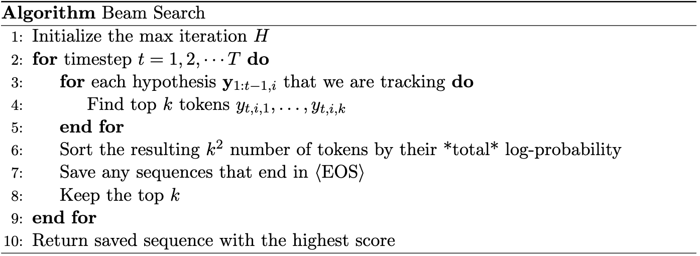
$\mathbf{Fig\ 6.}$ Beam Search pseudocode

This process is illustrated in the following figure:

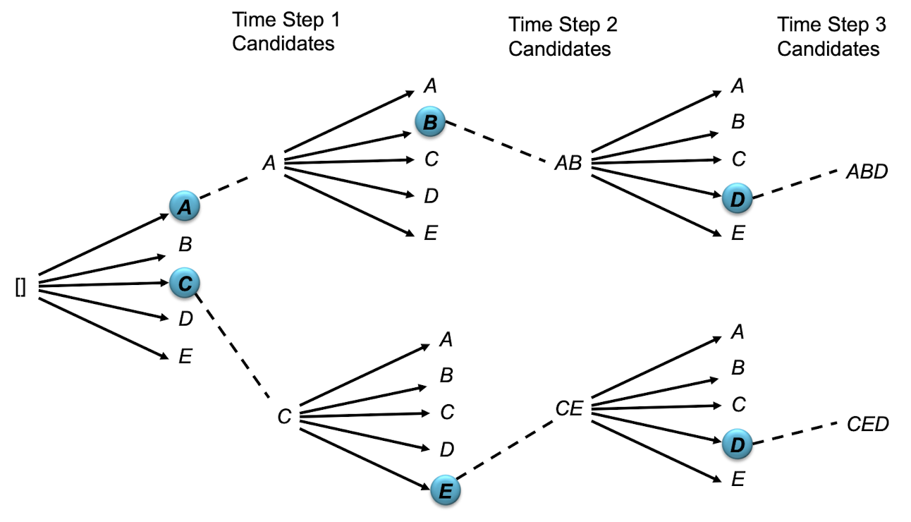
$\mathbf{Fig\ 7.}$ Beam Search ($k = 2$) illustration (source: [1])

Since the longer the sequence the lower its total score (more negative numbers added together), we compensate this disadvantage by dividing the length of the result sequence:

\[\begin{aligned} \text{score}(\mathbf{y}_{\text{i}, 1:T^\prime} \mid \mathbf{x}) = \frac{1}{T^\prime} \sum_{t=1}^{T^\prime} p(y_{\text{i}, t} \mid \mathbf{h}_t^{y_{\text{i}}}, \mathbf{h}_T^{\mathbf{x}}) \end{aligned}\]

Reference

[1] Kevin P. Murphy, Probabilistic Machine Learning: An introduction, MIT Press 2022.
[2] UC Berkeley CS182: Deep Learning, Lecture 11 by Sergey Levine
[3] Sutskever, Ilya, Oriol Vinyals, and Quoc V. Le. “Sequence to sequence learning with neural networks.” Advances in neural information processing systems 27 (2014).