
[DL] Attention Mechanisms
So far, we have considered the basic models of deep neural network. They have the ripple effect of solving numerous problems, but suffer for some problems. Consider the image classification task, worth a try with CNN architecture. What if the image is a lengthy image with too much white space? In that situation, CNN woule waste a lot of computing and time for convolving pointless space.

$\mathbf{Fig\ 1.}$ Image with redundant space
Let’s revisit to Seq2Seq model for Neural Machine Translation (NMT).

$\mathbf{Fig\ 2.}$ Seq2Seq model in NMT
Recall that it consists of encoder RNN and decoder RNN. Encoder RNN encodes source sequence and the last hidden state of the Encoder RNN is used to initialize the DecoderRNN. So, we can think the decoder is a conditional language model:
\[\begin{aligned} &p(y_1, \cdots, y_{T_t} | \mathbf{x} = (x_1, \cdots, x_{T_s})) \\ &= \prod_{t=1}^{T_t} p (y_t | y_{<t}, \mathbf{x}) \\ &= \prod_{t=1}^{T_t} p (y_t | h_t^y, h_T^{\mathbf{x}}) \end{aligned}\]The entire input sequence is compressed into a single vector $h_T^{\mathbf{x}}$ at the end of the encoder RNN. From this single compression vector, the decoder then need to extract necessary information at each decoding step. But, there may be a limit if the input sequence is too long to compress it in a single vector and it forms a bottleneck problem.
Attention mechanisms may be solutions for that, which are based on a neuro-architectural inductive bias for learning to search (where to attend). It can guide the model to solve
- Select a part in the input sequence that will provide useful information for the decoding of the current time step
- Encode information from the chosen part and provide it to the decoder
- Let the decoder utilize this information
Attention Mechanism
The basic of attention mechanisms is the operations between 3 vectors: key, query, value vector. Heuristically, key vector indicates what type of information that is encoded in the corresponding state, and query vector represents what we are searching for now. By checking the similarity between two vector, value vector corresponding to the certain key vector is selected. For instance, in web searching you can think these vector as
- Query: search word
- Key: title of the page
- Value: content of the page
Consider $m$ feature vectors, or values $\mathbf{V} \in \mathbb{R}^{m \times \text{D}{\text{V}}}$. And we find which feature vector to use by computing the similarity between the input query vector $\mathbf{q} \in \mathbb{R}^{\text{D}{\text{Q}}}$ and $m$ key vectors $\mathbf{K} \in \mathbb{R}^{m \times \text{D}_{\text{K}}}$. For example, if $\mathbf{q}$ is similar to $i$-th key vector, then we use $i$-th value vector. More generally, to make the operation differentiable, we may compute a combination of the values instead of taking one value vector:
\[\begin{aligned} \text{Attn}( \mathbf{q}, (\mathbf{k}_{1:m}, \mathbf{v}_{1:m}) ) = \sum_{i=1}^m \alpha_i (\mathbf{q}, \mathbf{k}_{1:m}) \mathbf{v}_i \end{aligned}\]where $\alpha_i$ is the function that compute attention weight (range is $[0, 1]$ and the sum of them is $1$). We can calculate these attention weights by measuring the similarity of query $\mathbf{q}$ and key $\mathbf{k_i}$ with a function called attetion score, $a: \mathbb{R}^{\text{D}{\text{Q}}} \times \mathbb{R}^{\text{D}{\text{K}}} \to \mathbb{R}$, and normalizing them. In mathematically,
\[\begin{aligned} \alpha_i (\mathbf{q}, \mathbf{k}_{1:m}) = \text{softmax}_i (a(\mathbf{q}, \mathbf{k}_1), \cdots, a(\mathbf{q}, \mathbf{k}_m)) = \frac{\text{exp}(a(\mathbf{q}, \mathbf{k}_i))}{\sum_{j=1}^m \text{exp}(a(\mathbf{q}, \mathbf{k}_j))} \end{aligned}\]

$\mathbf{Fig\ 3.}$ Attention mechanism
There are various way to select attention scoring function that computes the similarity of key and query vector, and also includes trainable parameters. Here are some examples:
Example: Attention in Seq2Seq
Now, let’s apply the mechanism into Seq2Seq model. The hidden states $h_1^{\mathbf{x}}, \cdots, h_{T_x}^{\mathbf{x}}$ of the input sequence becomes the keys and values. And, the current hidden states $h_t^y$ becomes the query.

$\mathbf{Fig\ 4.}$ Seq2Seq model
Although the hidden state of RNN is already passed through non-linear transformation, we can apply additional functions again to the state to create key, query, and value vectors, for instance learnable transformation $\mathbf{k}_t = \sigma( \mathbf{W} \mathbf{h}_t^{\mathbf{x}} + \mathbf{b})$. All computations of key, query, value, and also the output of decoder are left to the designer.
The following illustration shows the application of attention mechanism to Seq2Seq model:
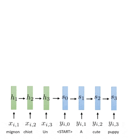
$\mathbf{Fig\ 5.}$ Illustration of attention in Seq2Seq model (source: [3])
Self-Attention
We now know how to use attention in seq2seq models, i.e., when we are given a query vector (e.g., from the decoder sequence). Then, can we make more general mechanism than attention with query? Can we use attention for non-seq2seq models without recurrent connections, e.g., sentence classification? How do we get the query vector?
One possible solution: A token in a sequence can serve as a query and apply attention to other tokens. It allows the encoder to attend itself. For instance, we may want to translate the sentence "The animal didn't cross the street because it was too tired". But, what does “it” in this sentence refer to? Street? Or, the animal? With self-attention, a model can search other input positions for hints that may help it create a more accurate encoding for this sentence.
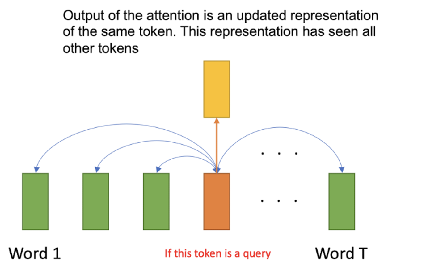
$\mathbf{Fig\ 6.}$ Apply attention to other tokens
Then, we can do this self-attention at every token in the input sequence in parallel. The one of the important property is, we don’t have to process in sequentially, which lets us attach MLP after the layer. For example, the following figure shows the simple self-attention network that classifies the positivity of sentence.
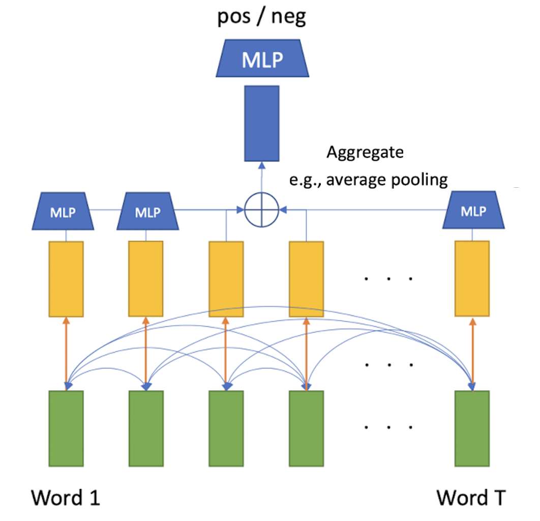
$\mathbf{Fig\ 7.}$ Parallel operation
Now, let’s get down to the details. A self-attention layer is specified by three learnable parameter matrices: $(\mathbf{W}^{\text{Q}}, \mathbf{W}^{\text{K}}, \mathbf{W}^{\text{V}})$ each of which for transforming the inputs $\mathbf{x}_i$ into query, key and value vectors, respectively. (Note that it is thanks to parallelism of self-attention) Suppose we have the $n$ number of input vectors with $d$ embedding dimensions, i.e., $\mathbf{X} \in \mathbb{R}^{n \times d}$. Then, we have $\mathbf{W}^{\text{Q}}, \mathbf{W}^{\text{K}} \in \mathbb{R}^{d \times d_k}$, and $\mathbf{W}^{\text{V}} \in \mathbb{R}^{d \times d_p}$.
\[\begin{aligned} &\mathbf{Q} = \mathbf{X} \mathbf{W}^{\text{Q}} \in \mathbb{R}^{n \times d_k} \\ &\mathbf{K} = \mathbf{X} \mathbf{W}^{\text{K}} \in \mathbb{R}^{n \times d_k} \\ &\mathbf{V} = \mathbf{X} \mathbf{W}^{\text{V}} \in \mathbb{R}^{n \times d_p} \end{aligned}\]And, we compute the attention weights with them. For instance, if we utilize scaled dot-product (divide a dot-product by $\sqrt{d_k}$ since dot product is summing $d_k$ values for each entry, to prevent the explosion):
\[\begin{aligned} \mathbf{Y} = \text{softmax} ( \frac{\mathbf{Q} \mathbf{K}^\top}{\sqrt{d_k}} , \text{dim} = 1) \mathbf{V} \end{aligned}\]There are much more powerfulness of Self-Attention compare to other layers:

$\mathbf{Fig\ 8.}$ Powefulness of self-attention
Multi-Head Self-Attention
We call a set of parameters $(\mathbf{W}^{\text{Q}}, \mathbf{W}^{\text{K}}, \mathbf{W}^{\text{V}})$ a head. A head determines a particular way to attend other tokens, and it could be helpful to represent multiple attention distributions of a token, by allowing multiple heads
Then we can construct multi-head self-attention by multiple weight sets $(\mathbf{W}_h^{\text{Q}}, \mathbf{W}_h^{\text{K}}, \mathbf{W}_h^{\text{V}})$ for $h = 1, \cdots, H$ with $H$ being the number of heads:

$\mathbf{Fig\ 9.}$ Multi-head self-attention
After the multiple self-attention, we may obtain $H$ attention-pooled value matrices $\mathbf{Z_1}, \cdots, \mathbf{Z_H}$. By concatenating & multiply with output weight matrix $\mathbf{W}^O$, the layer finally outputs the resulting matrices.
\[\begin{aligned} \mathbf{Z} = [\mathbf{Z}_1 \ \mathbf{Z}_2 \ \cdots \ \mathbf{Z}_H] \times \mathbf{W}^O \quad \text{ where } \quad \mathbf{Z}_i = \text{softmax} ( \frac{\mathbf{Q}_i \mathbf{K}_i^\top}{\sqrt{d_k}} , \text{dim} = 1) \mathbf{V}_i \end{aligned}\]The following figure shows the overview of the layer:

$\mathbf{Fig\ 10.}$ Pipeline of multi-head self-attention layer
Masked Self-Attention
Although self-attention allows a token to refer to all information of tokens in every position (i.e. from previous tokens, and also next tokens), it would be sometimes illegal in some applications with autoregressive property, for example language modeling. Recall the situation that we are training the Seq2Seq model. If the target sentence is "I love you", the decoder of Seq2Seq model should outputs each word by only attending to previous outputs.
To prevent model from looking ahead in the sequence, we can block the future tokens by masking with $- \infty$, but remaining only information of previous tokens:
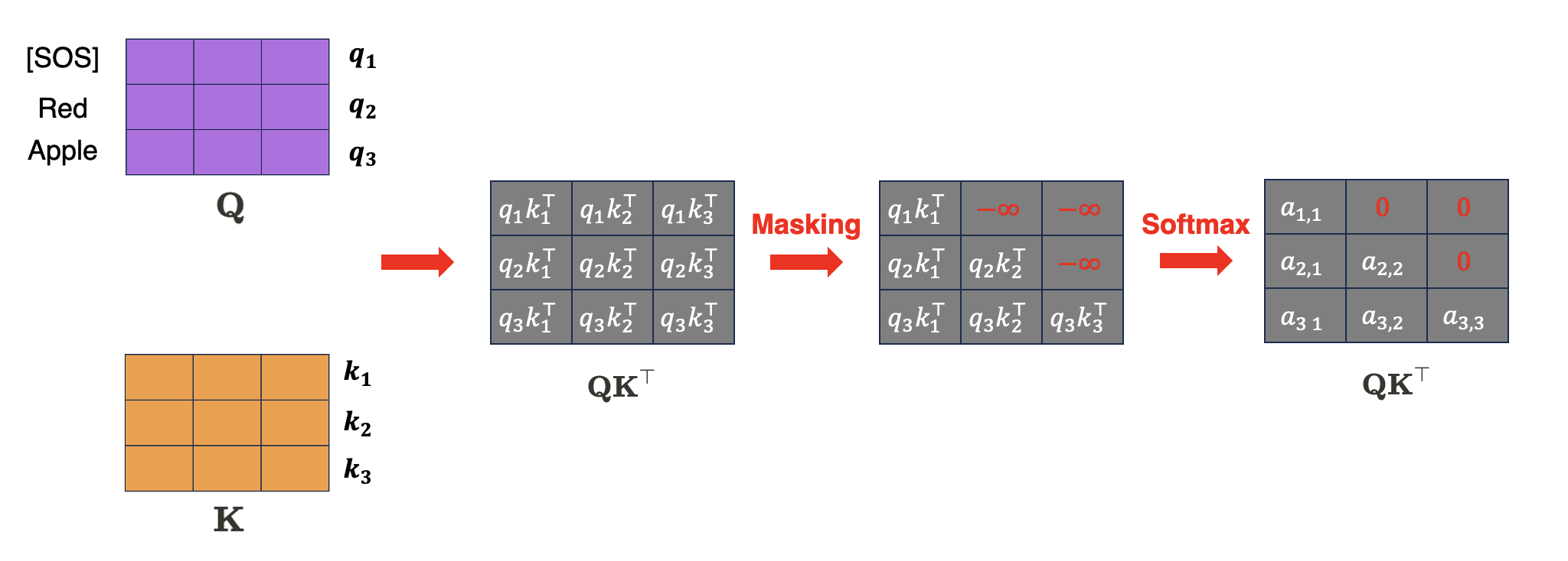
$\mathbf{Fig\ 11.}$ Masking self-attention
Power of Self-Attention
We close this post with a comparison between (1d) CNN, RNN, and Self-Attention layer. We focus on 3 aspects of three different models for mapping a sequence $\mathbf{x_{1:n}}$ to another sequence $\mathbf{y_{1:n}}$:
1. Complexity per Layer: The total computational complexity per layer
2. Sequential Operations: The minimum number of sequential operations required. Can quantify the amount of parallelizable computation.
3. Maximum Path Length: The expressive power quantified in terms of the length of the paths of computation signals to traverse in the network in order to connect any two inputs. Of course, the shorter the better.

$n$: sequence length, $d$: dimensionality of the input features, $k$: kernel size for convolution.
For (1D) CNN with kernel size $k$ and $d$ feature channels, the computation complexity is $O(knd^2)$, which can be done in parallel. And, we need to stack $n / k$ layers (or $\text{log}_k (n)$ if we used dilated convolution) to ensure all pairs can communicate. For example, we can see that $x_1$ and $x_5$ in the following figure can be connected together in the second layer.

For an RNN with a hidden state of size $d$, the complexity becomes $O(nd^2)$. Of course, RNN operation is an inherently sequential operation which cannot be parallelized, and the maximum path length is $O(n)$.

In the case of self-attention layer, every output is directly connected to every input, so the maximum path length is $O(1)$. However, the computational cost is $O(n^2d)$. But, it becomes much faster than RNN for short sequences $n « d$, which is common for various applications we, typically have $O(nd)$. For longer sequences, many fast versions of attention are studied recently.
https://theaisummer.com/self-attention/
Reference
[1] Kevin P. Murphy, Probabilistic Machine Learning: An introduction, MIT Press 2022.
[2] Stanford CS231n, Deep Learning for Computer Vision
[3] UC Berkeley CS182: Deep Learning, Lecture 11, 12 by Sergey Levine
[4] Zhang, Aston, et al. “Dive into deep learning.”, 11. Attention Mechanisms and Transformers
Leave a comment