[DL] Layer Normalization

Although batch normalization have various desirable properties for the training time of deep neural networks, it is not straightforward in case of RNN. For example, RNN, which is implemented by recurrent application of shared parameters, might have different statistics between the activations for each recurrent loop. It needs to compute and store separate statistics for each time step in a sequence, and it is problematic in terms of efficiency and maximum sentence length. Furthermore, if the model is trained with small batch size, e.g. model is distributed over machines.

Ba et al. 2016 proposed layer normalization, a simple normalization method but normalizes the features within a hidden layer unlike batch normalization.

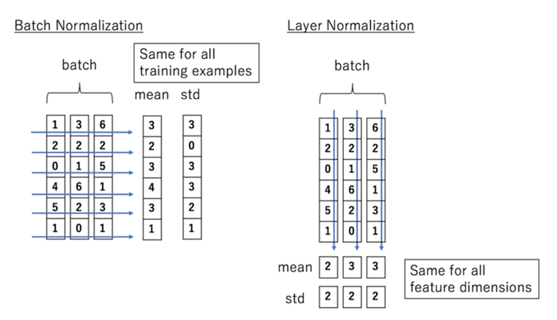
$\mathbf{Fig\ 1.}$ Batch Normalization v.s. Layer Normalization

For example, if each input has D features, i.e. D-dimension vector and the batch size is N, we normalize the vector along the length of the D-dimensional vector and not across the batch size N. Hence, the layer normalization does not introduce any new dependencies between training datapoints.

Notation

Consider $\ell$-th hidden layer in fully-connected network. Let $a^\ell$ be the summed inputs to the neurons and $w^\ell$, $b^\ell$ be the weights, bias parameter of $\ell$-layer respectively. In other words, if we denote $h^\ell$ as a outputs from the previous layer (input of $\ell$-th layer):

\[\begin{aligned} a_{i}^{\ell} = {w_{i}^{\ell}}^{\top} h^{\ell} \; \quad \; h_{i}^{\ell + 1} = f(a_{i}^{\ell} + b_{i}^{\ell}) \end{aligned}\]

where $f$ is an element-wise non-linearity. For example, the batch normalization normalizes and rescales $a^\ell_i$ by their means and variances under the distribution of data and rescale parameter $\mathbf{g}$:

\[\begin{aligned} \widetilde{a}^\ell_i = \mathbf{g} \cdot \frac{1}{\sigma_i^\ell} (a_i^\ell - \mu_i^\ell) \quad \text{ where } \quad \mu_i^\ell = \mathbb{E}_{\mathbf{x} \sim P(\mathbf{x})} [a_i^\ell] \quad \sigma_i^\ell = \sqrt{\mathbb{E}_{\mathbf{x} \sim P(\mathbf{x})} \left[ (a_i^\ell - \mu_i^\ell)^2 \right]} \end{aligned}\]

But the statistics are approximated by sample mean and variance along the batch \(\mathcal{B}_i = \{ a_{1, i}^\ell, \cdots, a_{\mid \mathcal{B} \mid, i}^\ell \}\), i.e.

\[\begin{aligned} \mu_i^\ell \approx \frac{1}{\mid \mathcal{B} \mid} \sum_{n = 1}^{\mid \mathcal{B} \mid} a_{n, i}^\ell \end{aligned}\]

---

Layer Normalization

The main problem of batch normalization is to prevent covariate shift i.e., the distribution of each layer’s inputs changes during training, which slows down the training by making it notoriously hard to train models.

Changes in the output of one layer will tend to cause highly correlated changes in the summed inputs to the next layer. I

Another viewpoint in layer normalization is, 여기들

\[\begin{aligned} \mu^\ell = \frac{1}{H} \sum_{i=1}^H a_i^\ell \quad \sigma^\ell = \sqrt{\frac{1}{H} \sum_{i=1}^H (a_i^\ell - \mu^\ell)^2} \end{aligned}\]

where $H$ is the number of hidden units, i.e. hidden dimension in a layer. Hence, it can performed without any constraint on the mini-batch size.

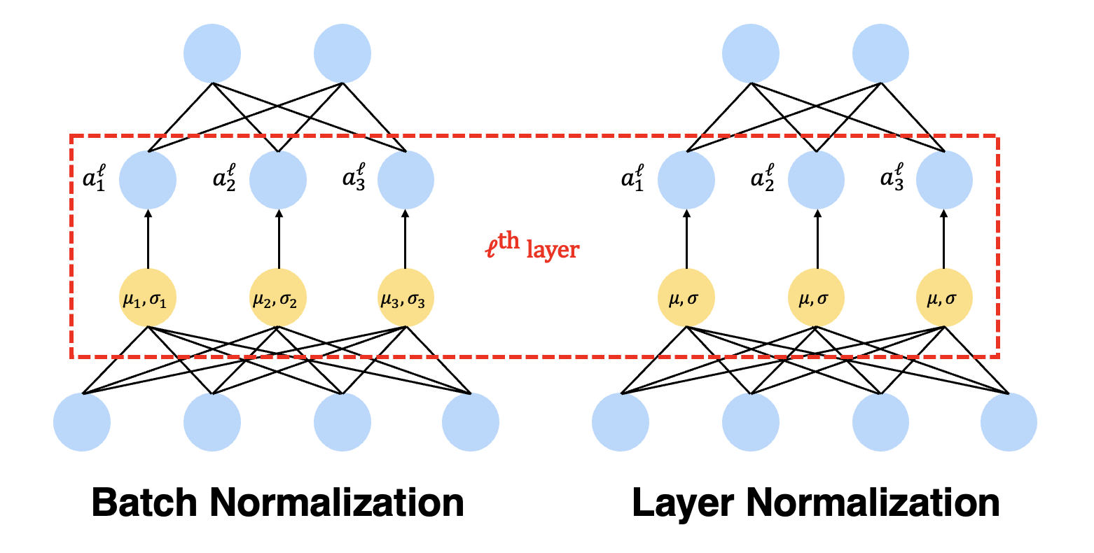
$\mathbf{Fig\ 2.}$ Batch Normalization v.s. Layer Normalization in MLP (source: current author)

Layer normalized RNN

In vanilla version of RNN, the summed inputs $\mathbf{a}^t$ is computed by the previous hidden states $\mathbf{h}^{t-1}$ and $\mathbf{x}^t$:

\[\begin{aligned} \mathbf{a}^t = W_{hh} h^{t-1} + W_{xh} \mathbf{x}^t \end{aligned}\]

Then the summed input is normalized, rescaled, recenetered and fed into a non-linearity for the next hidden state $\mathbf{h}^t$:

\[\begin{aligned} f \left[ \frac{\mathbf{g}}{\sigma^t} \odot (\mathbf{a}^t - \mu^t) + \mathbf{b} \right] \quad \text{ where } \quad \mu^t = \frac{1}{H} \sum_{i=1}^H a_i^t \quad \sigma^t = \sqrt{\frac{1}{H} \sum_{i=1}^H (a_i^t - \mu^t)^2} \end{aligned}\]

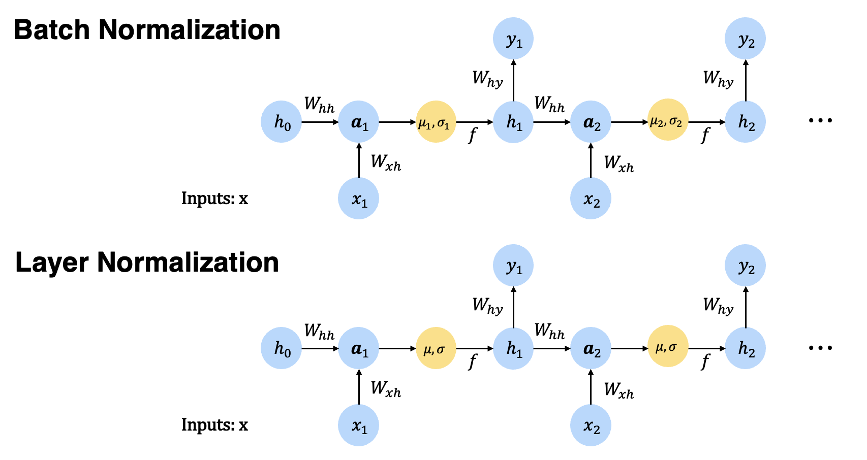
$\mathbf{Fig\ 3.}$ Batch Normalization v.s. Layer Normalization in RNN (source: current author)

Properties

Stable dynamics in RNN

RNN usually suffers from gradient vanishing and exploding. But if RNN is layer normalized, its dynamic of hidden states is much stable as the normalization terms make it invariant to r ~ 여기

Invariance under weights and data transformations

First of all, suppose $w_i$ is scaled by $\delta$ and shifted by scalar vector $\boldsymbol{\gamma}$. In other words, if $W$ denotes the original weight matrix of model, changed weight $W^\prime$ is computed by $W^\prime = \delta W + \mathbf{1} \boldsymbol{\gamma}^\top$.

Then, under layer normalization, the new output $\mathbf{h}^\prime$ will be same with the output before scaling and shift of weights $\mathbf{h}$:

\[\begin{aligned} \mathbf{h}^\prime & = f(\frac{\mathbf{g}}{\sigma^\prime} (W^\prime \mathbf{x} - \mu^\prime) + \mathbf{b}) = f(\frac{\mathbf{g}}{\sigma^\prime} ((\delta W + \mathbf{1} \boldsymbol{\gamma}^\top)\mathbf{x} - \mu^\prime) + \mathbf{b}) \\ & = f (\frac{\mathbf{g}}{\sigma} (W \mathbf{x} - \mu) + \mathbf{b}) = \mathbf{h} \end{aligned}\]

since the statistics of summed input $\mathbf{x}$ from the previous layer also scaled and shifted. But notice that it is not invariant to the individual scaling of the single weight vectors.

Next, suppose an individual datapoint $\mathbf{x}$ is rescaled and recented by $\delta$ and scalar vector $\boldsymbol{\gamma}$ of which dimension is equal to the dimension of datapoint, i.e. $\mathbf{x}^\prime = \delta \mathbf{x} + \boldsymbol{\gamma}$, then the mean and variance of summed input $w_i^\top \mathbf{x}^\prime$ will be $\mu^\prime = \delta \mu + w_i^\top \boldsymbol{\gamma}$ and $\sigma^\prime = \delta \sigma$. Hence,

\[\begin{aligned} h_i^\prime = f(\frac{g_i}{\sigma^\prime}(w_i^\top \mathbf{x}^\prime - \mu^\prime) + b_i) = f(\frac{g_i}{\delta \sigma}(\delta w_i^\top \mathbf{x} - \delta \mu) + b_i) = h_i \end{aligned}\]

Layer normalization is invariance to re-scaling and re-centering of single training case.

In summary,

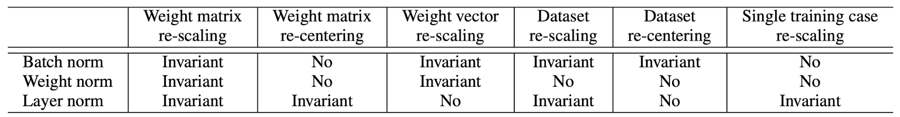
$\mathbf{Fig\ .}$ Invariance properties under the normalization methods.

Implicit early stopping effect on the weight vector

Before start, notice that KL divergence can be connected to a Riemannian metric called Fisher information metric:

\[\begin{aligned} \mathrm{D}_{\mathrm{KL}}[P(y \mid \mathbf{x} ; \theta) \| P(y \mid \mathbf{x} ; \theta+\delta)] \approx \frac{1}{2} \delta^{\top} F(\theta) \delta \end{aligned}\]

for small $\delta$

$\mathbf{Proof.}$

First of all, we claim that the negative expectation of Hessian equals to Fisher information matrix i.e. $F(\theta) = - \mathbb{E}_{x \sim p(x \mid \theta)} \left[ H(\text{log } p(x \mid \theta))\right]$. Note that

\[\begin{aligned} H(\text{log } p(x \mid \theta)) & = \nabla_\theta \frac{\nabla_\theta p(x \mid \theta)}{p(x \mid \theta)} \\ & = \frac{H ( p(x \mid \theta) )}{p(x \mid \theta)} - \left( \frac{\nabla_\theta p(x \mid \theta)}{p(x \mid \theta)} \right) \left( \frac{\nabla_\theta p(x \mid \theta)}{p(x \mid \theta)} \right)^\top \end{aligned}\]

By taking the expectation,

\[\begin{aligned} \mathbb{E}_{x \sim p(x \mid \theta)} \left[ H(\text{log } p(x \mid \theta))\right] & = \mathbb{E}_{x \sim p(x \mid \theta)}\left[\frac{H ( p(x \mid \theta) )}{p(x \mid \theta)}\right] - F(\theta) \\ & = \int \frac{H (p(x \mid \theta))}{p(x \mid \theta)} p(x \mid \theta) \cdot dx - F(\theta) \\ & = H ( \int p(x \mid \theta) dx) - F(\theta) \\ & = - F(\theta) \end{aligned}\]

Then, by 2nd order Taylor approximation:

\[\begin{aligned} \mathrm{D}_{\mathrm{KL}}[P(y \mid \mathbf{x} ; \theta) \| P(y \mid \mathbf{x} ; \theta+\delta)] & \approx \mathrm{D}_{\mathrm{KL}}[P(y \mid \mathbf{x} ; \theta) \| P(y \mid \mathbf{x} ; \theta)] + (\left. \nabla_{\theta^\prime} \mathrm{D}_{\mathrm{KL}}[P(y \mid \mathbf{x} ; \theta) \| P(y \mid \mathbf{x} ; \theta^\prime)] \right|_{\theta^\prime = \theta})^\top \delta + \frac{1}{2} \delta^\top F(\theta) \delta \\ & = (\left. \nabla_{\theta^\prime} \mathrm{D}_{\mathrm{KL}}[P(y \mid \mathbf{x} ; \theta) \| P(y \mid \mathbf{x} ; \theta^\prime)] \right|_{\theta^\prime = \theta})^\top \delta + \frac{1}{2} \delta^\top F(\theta) \delta \end{aligned}\]

From the fact that the expectation of score function $s(\theta) = \nabla_{\theta} \text{ log } p(x \mid \theta)$ is zero:

\[\begin{aligned} \mathbb{E}_{x \sim p(x \mid \theta)} \left[ s(\theta) \right] & = \int \nabla_{\theta} \text{ log } p(x \mid \theta) \cdot p(x \mid \theta) \cdot dx \\ & = \int \nabla_{\theta} p(x \mid \theta) \cdot dx \\ & = \nabla_{\theta} \int p(x \mid \theta) \cdot dx = 0 \end{aligned}\]

done.

\[\tag*{$\blacksquare$}\]

Hence Fisher Information Matrix defines the local curvature in distribution space for which KL-divergence is the metric.

The authors focused geometric analysis on the GLM. But the results can be easily applied to deep neural networks with block-diagonal approximation to the Fisher information matrix, where each block corresponds to the parameters for a single neuron. A GLM is a conditional version of an exponential family distribution, in which the natural parameters are a linear function of the input: [2, 3]

\[\begin{aligned} P( y \mid \mathbf{x} ; w, b, \sigma^2) = \text{exp} \left( \frac{y (w^\top \mathbf{x} + b) - \eta(w^\top \mathbf{x} + b)}{\sigma^2} + c(y, \sigma^2) \right) \end{aligned}\]

where the mean and variance is

\[\begin{aligned} &\mathbb{E} [y \mid \mathbf{x} ; w, b, \sigma^2] = \eta^\prime (w^\top \mathbf{x} + b) \overset{\Delta}{=} f(w^\top \mathbf{x} + b) \\ &\text{Var} (y \mid \mathbf{x} ; w, b, \sigma^2) = \eta^{\prime \prime} (w^\top \mathbf{x} + b) \sigma^2 = \sigma^2 f^\prime (w^\top \mathbf{x} + b) \end{aligned}\]

Here, $f$ is known as mean function, or transfer function that takes linear predictor output and transform it into a different scale, which is the analog of non-linearity in the neural network. For the derivation of mean and variance, refer to the following proof:

$\mathbf{Proof.}$

It can be obtained from the fact that the the first and second cumulant of the sufficient statistics in exponential family equal to derivatives of the log partition:

\[\begin{aligned} p(\mathbf{y} \mid \boldsymbol{\theta}) = h(\mathbf{y}) \text{exp} [\boldsymbol{\theta}^\top \mathcal{T}(\mathbf{y}) - A (\boldsymbol{\theta})] \quad \to \quad \mathbb{E}[\mathcal{T}(\mathbf{y})] = \nabla A(\boldsymbol{\theta}) \quad \text{Cov}[\mathcal{T}(\mathbf{y})] = \nabla^2 A(\boldsymbol{\theta}) \end{aligned}\] \[\tag*{$\blacksquare$}\]

And assume a $H$-dimensional output vector $\mathbf{y} = [y_1, y_2, \cdots, y_H]$ is modeled by $H$ independent GLMs with parameters $\boldsymbol{\theta} = [w_1^\top, b_1, \cdots, w_H^\top, b_H]$. Then the Fisher information matrix for this multi-dimensional GLM $F(\boldsymbol{\theta})$ is

\[\begin{aligned} F(\boldsymbol{\theta})=\underset{\mathbf{x} \sim P(\mathbf{x})}{\mathbb{E}}\left[\frac{\operatorname{Cov}[\mathbf{y} \mid \mathbf{x}]}{\sigma^4} \otimes\left[\begin{array}{cc} \mathbf{x} \mathbf{x}^{\top} & \mathbf{x} \\ \mathbf{x}^{\top} & 1 \end{array}\right]\right] \end{aligned}\]

Note that Kronecker product $\otimes: \mathbb{R}^{m \times n} \times \mathbb{R}^{p \times q} \to \mathbb{R}^{pm \times qn}$ is defined as

\[\begin{aligned} \mathbf{A} \otimes \mathbf{B}=\left[\begin{array}{ccc} a_{11} \mathbf{B} & \cdots & a_{1 n} \mathbf{B} \\ \vdots & \ddots & \vdots \\ a_{m 1} \mathbf{B} & \cdots & a_{m n} \mathbf{B} \end{array}\right] \end{aligned}\]

$\mathbf{Proof.}$ Derivation of $F(\boldsymbol{\theta})$

Recall that the definition of Fisher information is defined as

\[\begin{aligned} F(\theta) = \mathbb{E}_{\mathbf{x} \sim p(\mathbf{x}), \mathbf{y} \sim p(\mathbf{y})} \left[ \frac{\partial \text{ log } P (y \mid \mathbf{x}; \theta)}{\partial \theta} \frac{\partial \text{ log } P (y \mid \mathbf{x}; \theta)}{\partial \theta}^\top \right] \end{aligned}\]

Since $P( y \mid \mathbf{x} ; w, b, \sigma^2) = \text{exp} \left( \frac{y (w^\top \mathbf{x} + b) - \eta(w^\top \mathbf{x} + b)}{\sigma^2} + c(y, \sigma^2) \right)$, for $\mathbf{y} = [y_1, y_2, \cdots, y_H]$,

\[\begin{aligned} & \frac{\partial \text{ log } P(\mathbf{y} \mid \mathbf{x}\; ; \; \boldsymbol{\theta}, \sigma^2)}{\partial \boldsymbol{\theta}} = \frac{\partial}{\partial \boldsymbol{\theta}} \left[ \sum_{i=1}^H \frac{y_i (w_i^\top \mathbf{x} + b_i) - \eta(w_i^\top \mathbf{x} + b_i)}{\sigma^2} + c(y_i ; \sigma^2) \right] \\ & = \left[ \frac{y_1 \mathbf{x}}{\sigma^2} - \frac{\mathbf{x} \eta^\prime (w_1^\top \mathbf{x} + b_1)}{\sigma^2}, \; \frac{y_1}{\sigma^2} - \frac{\eta^\prime (w_1^\top \mathbf{x} + b_1)}{\sigma^2}, \; \cdots \; ,\frac{y_H \mathbf{x}}{\sigma^2} - \frac{\mathbf{x} \eta^\prime (w_H^\top \mathbf{x} + b_H)}{\sigma^2}, \; \frac{y_H}{\sigma^2} - \frac{\eta^\prime (w_H^\top \mathbf{x} + b_H)}{\sigma^2} \right]^\top \\ & = \left[ \frac{y_1 \mathbf{x}}{\sigma^2} - \frac{\mathbf{x} \mathbb{E}[y_1 \mid \mathbf{x}]}{\sigma^2}, \; \frac{y_1}{\sigma^2} - \frac{\mathbb{E}[y_1 \mid \mathbf{x}]}{\sigma^2}, \; \cdots \; ,\frac{y_H \mathbf{x}}{\sigma^2} - \frac{\mathbf{x} \mathbb{E}[y_H \mid \mathbf{x}]}{\sigma^2}, \; \frac{y_H}{\sigma^2} - \frac{\mathbb{E}[y_H \mid \mathbf{x}]}{\sigma^2} \right]^\top \\ \end{aligned}\]

Hence,

\[\begin{aligned} F(\boldsymbol{\theta}) & = \mathbb{E} [ \begin{bmatrix} \frac{\mathbf{x}}{\sigma^2} (y_1 - \mathbb{E}[y_1 \mid \mathbf{x}]) \\ \frac{1}{\sigma^2} (y_1 - \mathbb{E}[y_1 \mid \mathbf{x}]) \\ \vdots \end{bmatrix} \left[\frac{\mathbf{x}^\top}{\sigma^2} (y_1 - \mathbb{E}[y_1 \mid \mathbf{x}]) \quad \frac{1}{\sigma^2} (y_1 - \mathbb{E}[y_1 \mid \mathbf{x}]) \quad \cdots \quad \right]] \\ & = \mathbb{E} [ \frac{1}{\sigma^4} \begin{bmatrix} \mathbf{x} (y_1 - \mathbb{E}[y_1 \mid \mathbf{x}]) \\ y_1 - \mathbb{E}[y_1 \mid \mathbf{x}] \\ \vdots \end{bmatrix} \left[ \mathbf{x}^\top (y_1 - \mathbb{E}[y_1 \mid \mathbf{x}]) \quad y_1 - \mathbb{E}[y_1 \mid \mathbf{x}] \quad \cdots \quad \right]] \\ & = \underset{\mathbf{x} \sim P(\mathbf{x})}{\mathbb{E}}\left[\frac{\operatorname{Cov}[\mathbf{y} \mid \mathbf{x}]}{\sigma^4} \otimes\left[\begin{array}{cc} \mathbf{x} \mathbf{x}^{\top} & \mathbf{x} \\ \mathbf{x}^{\top} & 1 \end{array}\right]\right] \end{aligned}\] \[\tag*{$\blacksquare$}\]

Consider the case of normalized GLMs, which are obtained by applying the normaliztion to the summed inputs $a_i = w_i^\top \mathbf{x}$ through statistics of layer $\mu_i$ and $\sigma_i$. Denote $\bar{F}$ as its Fisher information matrix with the additional rescale parameter $\mathbf{g} = [g_1, \cdots, g_H]^\top$. Then, we can derive the following equation in the analogous way ($\phi = \sigma^2$):

\[\begin{gathered} \bar{F}(\boldsymbol{\theta})=\left[\begin{array}{ccc} \bar{F}_{11} & \cdots & \bar{F}_{1 H} \\ \vdots & \ddots & \vdots \\ \bar{F}_{H 1} & \cdots & \bar{F}_{H H} \end{array}\right], \quad \bar{F}_{i j}=\underset{\mathbf{x} \sim P(\mathbf{x})}{\mathbb{E}}\left[\frac{\operatorname{Cov}\left[y_i, y_j \mid \mathbf{x}\right]}{\phi^2}\left[\begin{array}{ccc} \frac{g_i g_j}{\sigma_i \sigma_j} \chi_i \chi_j^{\top} & \chi_i \frac{g_i}{\sigma_i} & \chi_i \frac{g_i\left(a_j-\mu_j\right)}{\sigma_i \sigma_j} \\ \chi_j^{\top} \frac{g_j}{\sigma_j} & 1 & \frac{a_j-\mu_j}{\sigma_j} \\ \chi_j^{\top} \frac{g_j\left(a_i-\mu_i\right)}{\sigma_i \sigma_j} & \frac{a_i-\mu_i}{\sigma_i} & \frac{\left(a_i-\mu_i\right)\left(a_j-\mu_j\right)}{\sigma_i \sigma_j} \end{array}\right]\right] \\ \chi_i=\mathbf{x}-\frac{\partial \mu_i}{\partial w_i}-\frac{a_i-\mu_i}{\sigma_i} \frac{\partial \sigma_i}{\partial w_i} . \end{gathered}\]

$\mathbf{Proof.}$ Derivation of $\bar{F}_{ij}$

Note that

\[\begin{aligned} & \frac{\partial}{\partial w_i} \left [\frac{g_i}{\sigma_i} (w_i^\top \mathbf{x} - \mu_i) + b_i \right] = \frac{g_i}{\sigma_i} (\mathbf{x} - \frac{\partial \mu_i}{\partial w_i} - \frac{a_i - \mu_i}{\sigma_i} \frac{\partial \sigma_i}{\partial w_i}). \end{aligned}\]

Thus, let’s denote $\chi_i = \mathbf{x} - \frac{\partial \mu_i}{\partial w_i} - \frac{a_i - \mu_i}{\sigma_i} \frac{\partial \sigma_i}{\partial w_i}$.

Since $P( y \mid \mathbf{x} \; ; \; \theta, \phi) = \text{exp} \left( \frac{y (\frac{g}{\sigma} (w^\top \mathbf{x} - \mu) + b) - \eta(\frac{g}{\sigma} (w^\top \mathbf{x} - \mu) + b)}{\phi} + c(y, \phi) \right)$, for $\mathbf{y} = [y_1, y_2, \cdots, y_H]$

\[\begin{aligned} & \frac{\partial \text{ log } P(\mathbf{y} \mid \mathbf{x}\; ; \; \boldsymbol{\theta}, \sigma^2)}{\partial \boldsymbol{\theta}} = \frac{\partial}{\partial \boldsymbol{\theta}} \left[ \sum_{i=1}^H \frac{y_i (\frac{g_i}{\sigma_i} (w_i^\top \mathbf{x} - \mu_i) + b_i) - \eta(\frac{g_i}{\sigma_i} (w_i^\top \mathbf{x} - \mu_i) + b_i)}{\phi} + c(y_i ; \phi) \right] \\ \end{aligned}\]

For $i = 1, \cdots, H$, the $i$-th block of the vector can be written as

\[\begin{aligned} \left( \frac{\partial \text{ log } P(\mathbf{y} \mid \mathbf{x}\; ; \; \boldsymbol{\theta}, \sigma^2)}{\partial \boldsymbol{\theta}} \right)_{i} & = \begin{bmatrix} \frac{\frac{g_i}{\sigma_i} y_i \chi_i}{\phi} - \frac{\frac{g_i}{\sigma_i} \chi_i \eta^\prime (\frac{g_i}{\sigma_i} (w_i^\top \mathbf{x} - \mu_i) + b_i)}{\phi} \\ \frac{y_i}{\phi} - \frac{\eta^\prime (w_i^\top \mathbf{x} + b_i)}{\phi} \\ \frac{\frac{y_i}{\sigma_i} (w_i^\top \mathbf{x} - \mu_i)}{\phi} - \frac{\frac{w_i^\top \mathbf{x} - \mu_i}{\sigma_i} \eta^\prime (\frac{g_i}{\sigma_i} (w_i^\top \mathbf{x} - \mu_i) + b_i)}{\phi} \end{bmatrix} \\ & = \frac{1}{\phi} \begin{bmatrix} \frac{g_i y_i \chi_i}{\sigma_i} - \frac{g_i \mathbb{E}[y_i \mid \mathbf{x}] \chi_i}{\sigma_i} \\ y_i - \mathbb{E}[y_i \mid \mathbf{x}] \\ y_i \frac{(a_i - \mu_i)}{\sigma_i} - \frac{(a_i - \mu_i)}{\sigma_i} \mathbb{E}[y_i \mid \mathbf{x}] \end{bmatrix} \\ \end{aligned}\]

Hence,

\[\begin{aligned} \bar{F}_{ij} & = \frac{1}{\phi^2} \mathbb{E} [ \begin{bmatrix} \frac{g_i}{\sigma_i} (y_i - \mathbb{E}[y_i \mid \mathbf{x}]) \chi \\ y_i - \mathbb{E}[y_i \mid \mathbf{x}] \\ \frac{a_i - \mu_i}{\sigma_i} (y_i - \mathbb{E}[y_i \mid \mathbf{x}]) \end{bmatrix} \left[\frac{g_j}{\sigma_j} (y_j - \mathbb{E}[y_j \mid \mathbf{x}]) \chi_j^\top \quad y_j - \mathbb{E}[y_j \mid \mathbf{x}] \quad \frac{a_j - \mu_j}{\sigma_j} (y_j - \mathbb{E}[y_j \mid \mathbf{x}]) \right] ] \\ & = \underset{\mathbf{x} \sim P(\mathbf{x})}{\mathbb{E}}\left[\frac{\operatorname{Cov}(y_i, y_j \mid \mathbf{x})}{\phi^2} \cdot \left[\begin{array}{ccc} \frac{g_i g_j}{\sigma_i \sigma_j} \chi_i \chi_j^\top & \chi_i \frac{g_i}{\sigma_i} & \chi_i \frac{g_i (a_j - \mu_j)}{\sigma_i \sigma_j} \\ \chi_j^\top \frac{g_j}{\sigma_j} & 1 & \frac{a_j - \mu_j}{\sigma_j} \\ \chi_j^\top \frac{g_j (a_i - \mu_i)}{\sigma_i \sigma_j} & \frac{a_i - \mu_i}{\sigma_i} & \frac{(a_i - \mu_i) (a_j - \mu_j)}{\sigma_i \sigma_j} \end{array}\right]\right] \end{aligned}\] \[\tag*{$\blacksquare$}\]

Here, unlike standard GLM, $\bar{F}_{ij}$ along the weight vector $w_i$ direction is scaled by the rescale parameter $g_i$ and normalization scalar $\sigma_i$. This indicates that for the same parameter update in the normalized model, the norm of the weight vector effectively controls the learning rate for the weight vector. In other words, the normalization methods have an implicit early stopping effect on the weight vectors and help to stabilize learning towards convergence.

For example, if the norm of the weight $w_i$ grows twice as large, due to layer normalization and its invariance, normalized GLM still yields the same output, but the curvature along the $w_i$ direction will be decreased by $\frac{1}{2}$ since $\sigma_i$ is also twice as large.

Reference

[1] Ba, Jimmy Lei, Jamie Ryan Kiros, and Geoffrey E. Hinton. “Layer normalization.” arXiv preprint arXiv:1607.06450 (2016).
[2] Kevin P. Murphy, Probabilistic Machine Learning: An introduction, MIT Press 2022., 12. Generalized Linear Models
[3] Benoit Sanchez, Why do we assume the exponential family in the GLM context?