
[DL] Transformer
Transformer
Overall architecture of Transformer (source)
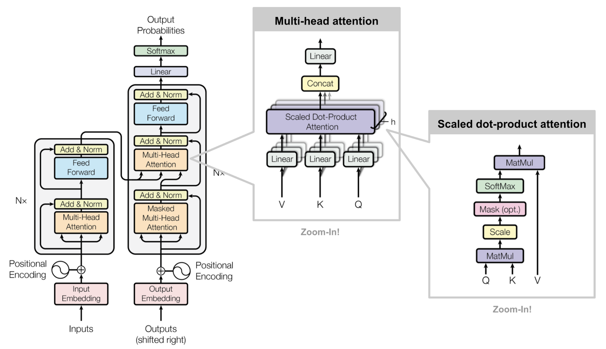
In this post, we will look at Transformer, a state-of-the-art model proposed in the paper Attention is All You Need. Transformer is a model originally proposed for machine translation using multilayer self-attention but it does not use any RNN or CNN. The central ideas of the Transformer model is quite general, so it is now replacing almost all sequential models using RNNs and even image modeling by replacing CNNs.
A Transformer block has the following architecture:
- Multi-Head Attention
- Residual + Layer Normalization
- Feed-Forward Network (= MLP)
- Residual + Layer Normalization

$\mathbf{Fig\ 1.}$ Transformer Block [2]
And we usually stack multiple Transformer blocks for modeling. For example, the following figure shows the Seq2Seq model, but Transformer Architecture is utilized in the original paper.

$\mathbf{Fig\ 2.}$ Transformer-based Encoder & Decoder model (source: Vaswani et al.)
Positional Encoding
The architecture utilizes the additional technique called positional encoding for the first encoder, which assigns position information to the input.
Consider permuting the input vectors. Then, the components of self-attention layer (queries, keys, similarities, attention weights, etc.) will be same but just permuted. That means, self-attention works on sets of vectors and ignores position information. While this orderless-ness is the key property enabling parallel computation, but losing the order information is critical in a few applications like NLP.
To make processing position-aware, one possible way is to represent each position by an integer. For example, we can modify the input $x_t$ as
\[\begin{aligned} \widetilde{x}_t = \begin{bmatrix} x_t \\ t \end{bmatrix} \end{aligned}\]But, neural networks usually cannot handle integers and boundary in the value and the magnitude is unlimited. A float between 0 ~ 1 friendly may be preferred, but, you need to know the length of the sequence beforehand. Also, it is not a great idea as absolute position is less important than relative position. For example, consider two equivalent sentences "I walk my dog every day" and "Everyday I walk my dog".
Instead of it, we want to represent position in a way that tokens with similar relative position have similar encoding. To do so, we concatenate input with positional encoding, a frequency-based representation of the position.
With $i$ for token index and $j$ for embedding index, it is computed as follows:
where $C = 10000$ corresponds to some maximum sequence length. The following figure visualizes 128-dimensional positional encoding for a sentence with the maximum length of $C = 50$. Each row represents the embedding vector:

$\mathbf{Fig\ 3.}$ Illustration of positional encoding (source)
To obtain the input embedding for self-attention, the position encoding and the token embedding are simply element-wise summed. Thus it enables a model to address lack of sequence information in the input.

$\mathbf{Fig\ 4.}$ Aggregating position encoding to the input (source)
Intuition
Recall that the frequency of sine & cosine functions, for example the frequency of $f(x) = \text{sin}(x / a)$ is $2\pi a$. As it has much shorter frequency for smaller $a$, the deeper embedding dimension of token is, the longer frequency of positional encoding is. It is somewhat straightforward: it coincides with the property of binary encoding that frequency varies from the dimension. Suppose the integer for position is encoded into binary indexing. We see that the LSB toggles the fastest (has highest frequency), whereas the MSB toggles the slowest.
To smooth the integer encoding, we may exploit sine function based encoding, which is one of the most easiest to analyze among periodic functions. Since it has a value between -1 and 1, it is desirable to the neural network.
Let’s plot encoded values of total 3 dimensions if each position in the dimension is represented by a sine function with a period of $4 \pi$, $8 \pi$ and $16\pi$:
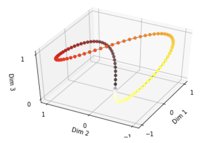
$\mathbf{Fig\ 5.}$ Sinusoidal encoding (source: Jonathan Kernes's Post)
The 3D graph above shows that the space represented by the three sine functions is a closed system because the period of each dimension follows the shape of $2^n \pi$. Our design of positional encoding seems nice to not only avoid that, but also the frequencies are monotone along the embedding dimension that it does not sidetrack from our intuition in binary encoding.
Finally, the reason why sine and cosine alternate along the embedding dimension is that it leads to some desirable property that enables the model to learn relative position on the input. And we will delve into this property in the next subsection. In addition, using them together helps each position to be more clearly distinguished:
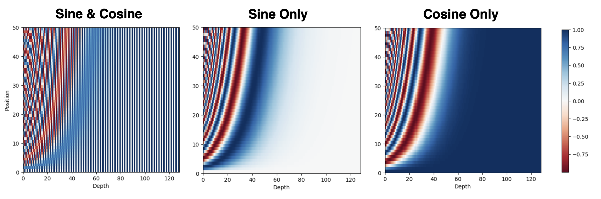
$\mathbf{Fig\ 6.}$ Comparison between position encodings with different version (source: current author)
Here is a notebook for experiment:
For more details about positional encoding, I recommend you to refer Amirhossein Kazemnejad’s Blog and Jonathan Kernes’s Post.
Learn to attend by relative positions
The advantages of the positional encoding is that it can be applied for arbitrary length inputs up to $T \leq C$ in contrast to a learned embedding. But most desirable property is, thanks to sinusoidal bases and mixed use of sine and cosine, the encoding of one position is linearly predictable (and it is a concept similar to the relative distance), i.e., $p_{t + \phi} = f(p_t)$ for linear transformation $f$:
Hence, it would allow the Transformer (especially self-attention, which only involves linear transformations) to easily learn to attend by relative positions, since for any fixed offset $k$, \(\text{PE}_{\text{pos}+k}\) can be represented as a linear function of \(\text{PE}_{\text{pos}}\). (Furthermore, for small $\phi$, $p_{t+ \phi} \approx p_t$.)
Position-wise Feed-Forward Networks
Since self-attention layers basically consist of linear operations, it is not adept at complex processing the information. So as to add more expressivity to the post-processing of attention, the multi-head self-attention layer in Transformer block is followed by some non-linear transformations of fully-connected layer:
\[\begin{aligned} \text{FFN}(x) = \text{ReLU}(x W_1 + b_1) W_2 + b_2 = \text{max}(0, xW_1 + b_1) W_2 + b_2 \end{aligned}\]but applied to each position separately and identically. Thus these are referred to as position-wise feed-forward networks.
Add & Layer Normalization
In the diagram of Transformer, Add & Norm are divided into two separate steps:
- Add:
residual connection - Norm:
layer normalization
These techniques help the model to be trained well by preventing degradation problem when blocks are deeply stacked and stabilizing the training, but without changes to the core of the model.
Masked Decoding
The authors also modify the self-attention layer in the decoder stack to prevent positions from attending to subsequent positions: Masked multi-head attention. This masking not only preserves paralleism in training but also ensures that the predictions for position $i$ can depend only on the known outputs at positions less than $i$. Hence it prevents the cheating in the decoder.
Let’s consider an example for further understanding, assume that we are training the machine translator, English to Spanish, with Transformer-based Seq2Seq model. Suppose the following training data is given to the model:
Eng: "How are you today"
Span: "Cómo estás hoy"
Then, "How are you today" will be given to the input of encoder, and "Cómo estás hoy" will be a target sentence of the decoder. As we know the expected target of decoder, there is a chance to preserve the parallelism in training thanks to self-attention layers [8]. Note that our tasks are to train the following 4 operations:
- Operation 1
-
Input: \(\mathbf{x}_1 =\)
<SOS> -
Target: \(\mathbf{y}_1 =\)
"Cómo"
-
Input: \(\mathbf{x}_1 =\)
- Operation 2
-
Input: \(\mathbf{x}_2 =\)
"Cómo" -
Target: \(\mathbf{y}_2 =\)
"estás"
-
Input: \(\mathbf{x}_2 =\)
- Operation 3
-
Input: \(\mathbf{x}_3 =\)
"estás" -
Target: \(\mathbf{y}_3 =\)
"hoy"
-
Input: \(\mathbf{x}_3 =\)
- Operation 4
-
Input: \(\mathbf{x}_4 =\)
"hoy" -
Target: \(\mathbf{y}_4 =\)
<EOS>
-
Input: \(\mathbf{x}_4 =\)
Then, by feeding \(\mathbf{X} = [ \mathbf{x}_1 \; \mathbf{x}_2 \; \mathbf{x}_3 \; \mathbf{x}_4]^\top\) to the decoder input and replacing multi-head attention in the first layer of decoder block with masked multi-head attention, it enables parallel training, preserving the auto-regressive property of decoder simultaneously.
Combining Encoder & Decoder
To connect the encoder and decoder, we employs a technique called cross attention. Let $N$ be the number of encoder (then the number of decoder block is also $N$). Denote \(\mathbf{e}_t^\ell\) as hidden state of input token $x_t$ in $\ell$-th layer of encoder. Then \(\mathbf{e}_1^N, \dots, \mathbf{e}_T^N\) are output vectors of encoder and define
\[\begin{aligned} \mathbf{E} = \begin{bmatrix} \mathbf{e}_1^N \\ \mathbf{e}_2^N \\ \vdots \\ \mathbf{e}_T^N \\ \end{bmatrix} \end{aligned}\]and for outputs \(\mathbf{d}_1^\ell, \mathbf{d}_1^\ell, \dots, \mathbf{d}_1^\ell\) of masked multi-head attention (followed by adding & layer normalization) in each decoder block $\ell = 1, 2, \dots, N$, define
\[\begin{aligned} \mathbf{D} = \begin{bmatrix} \mathbf{d}_1^\ell \\ \mathbf{d}_2^\ell \\ \vdots \\ \mathbf{d}_T^\ell \\ \end{bmatrix} \end{aligned}\]Encoder of Transformer passes $\mathbf{E}$ to each decoder block as key and value of multi-head attention in each decoder layer. And it is straightforward that the query will be $\mathbf{D}$. Since the source of query, key and value are different, it is often referred to as multi-head cross attention: for $h = 1, \dots, H$,
\[\begin{aligned} & \mathbf{Q}_h = \mathbf{D} \mathbf{W}_h^{\text{Q}} \in \mathbb{R}^{n \times d_k} \\ & \mathbf{K}_h = \mathbf{E} \mathbf{W}_h^{\text{K}} \in \mathbb{R}^{n \times d_k} \\ & \mathbf{V}_h = \mathbf{E} \mathbf{W}_h^{\text{V}} \in \mathbb{R}^{n \times d_p} \\ & \mathbf{Z}_h = \text{softmax}(\frac{\mathbf{Q}_h \mathbf{K}_h^\top}{\sqrt{d_k}}, \text{dim} = 1) \mathbf{V}_h & \mathbf{Z} = [\mathbf{Z}_1 \ \mathbf{Z}_2 \ \cdots \ \mathbf{Z}_H] \times \mathbf{W}^{\text{O}} \end{aligned}\]The following figure shows the illustration of entire encoder-decoder model based on Transformer block:
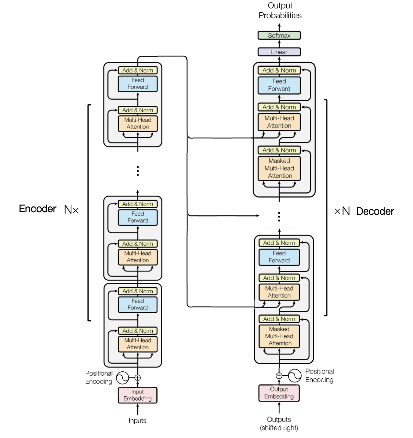
$\mathbf{Fig\ 6.}$ Encoder-Decoder Transformer (source: current author)
Reference
[1] Kevin P. Murphy, Probabilistic Machine Learning: An introduction, MIT Press 2022.
[2] Stanford CS231n, Deep Learning for Computer Vision
[3] The Illustrated Transformer
[4] Vaswani, Ashish, et al. “Attention is all you need.” Advances in neural information processing systems 30 (2017).
[5] Transformer Architecture: The Positional Encoding
[6] UC Berkeley CS182: Deep Learning, Lecture 12 by Sergey Levine
[7] Zhang, Aston, et al. “Dive into deep learning.”, 11. Attention Mechanisms and Transformers
[8] CodeEmporium, Why masked Self Attention in the Decoder but not the Encoder in Transformer Neural Network?
Leave a comment