[DL] Transposed Convolution

Transposed Convolution

---

Tranposed Convolution is one of upsampling techniques including unpooling which is frequently used in semantic segmentation. There are many different terminologies that point the transposed convolution operation, such as deconvolution, upconvolution, frationally strided convolution, and backward convolution.

If $N \times N$ input feature map passes through convolution layer of $K \times K$ kernel with stride of $S$ and $P$ padding, then the output size of this layer is shrinked to $(\lfloor \frac{N - K + 2P}{S} \rfloor + 1) \times (\lfloor \frac{N - K + 2P}{S} \rfloor + 1)$. As we can conjecture from the word “transpose”, transposed convolution is an operation designed in order to roll back the shrinked size to the input size.

Matrix view of convolution

Let’s take for example the convolution operation of $4 \times 4$ input and $3 \times 3$ kernel with stride $1$ and no padding.

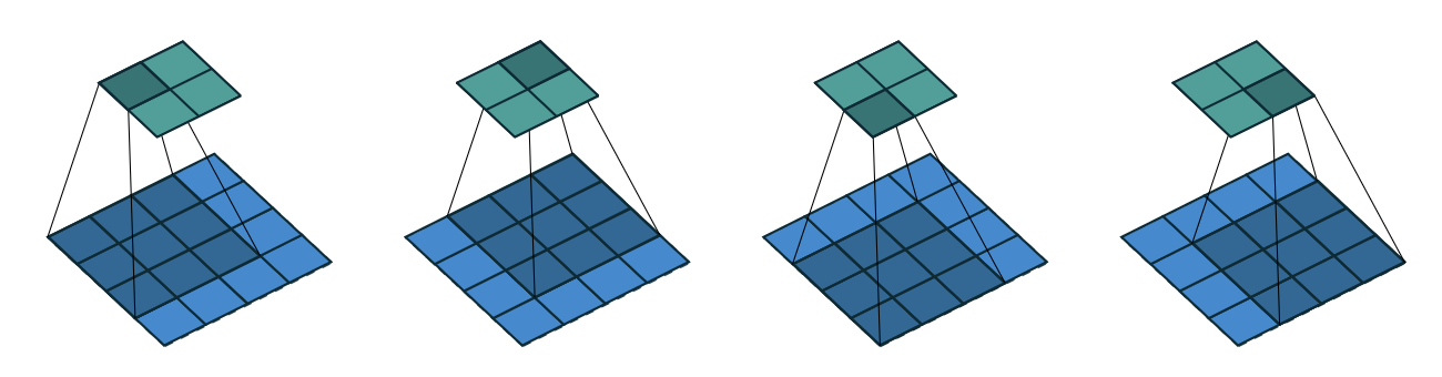
$\mathbf{Fig\ 1.}$ Convolution operation with $k = 4$, $s = 3$, $p = 0$

If the input and output feature maps are flattened into vectors $\mathbf{x}$ from left to right, top to bottom, the convolution kernel can be represented as a sparse matrix $\mathbf{C}$:

\[\left(\begin{array}{cccccccccccccccc} w_{0,0} & w_{0,1} & w_{0,2} & 0 & w_{1,0} & w_{1,1} & w_{1,2} & 0 & w_{2,0} & w_{2,1} & w_{2,2} & 0 & 0 & 0 & 0 & 0 \\ 0 & w_{0,0} & w_{0,1} & w_{0,2} & 0 & w_{1,0} & w_{1,1} & w_{1,2} & 0 & w_{2,0} & w_{2,1} & w_{2,2} & 0 & 0 & 0 & 0 \\ 0 & 0 & 0 & 0 & w_{0,0} & w_{0,1} & w_{0,2} & 0 & w_{1,0} & w_{1,1} & w_{1,2} & 0 & w_{2,0} & w_{2,1} & w_{2,2} & 0 \\ 0 & 0 & 0 & 0 & 0 & w_{0,0} & w_{0,1} & w_{0,2} & 0 & w_{1,0} & w_{1,1} & w_{1,2} & 0 & w_{2,0} & w_{2,1} & w_{2,2} \end{array}\right)\]

and convolution can be simply computed by matrix multiplication $\mathbf{C} \mathbf{x}$, so that the backward pass is easily obtained by transposing $\mathbf{C}$ by simple matrix calculus. Hence the gradient will be backpropagated by multiplying the loss with $\mathbf{C}^\top$.

Notably, it is a well-known fact that a CNN is equivalent to a fully connected network, with sparse connections and weight sharing.

Transposed convolution

Transposed convolution is implemented by swapping the forward and backward passes of the original convolution. So with respect to the matrix representation of convolution, it is possible to implement a transposed convolution with transposed matrix of kernel. In other words, the transposed convolution operation can be thought of as the gradient of corresponding convolution with regard to its input. To my knowledge, TensorFlow adopts such an approach.

Emulation with direct convolution

Through the matrix representation, it is easy to know the logic and way to implement transposed convolution but it is not straightforward to find intuition and visualize it just like convolution operation.

Hence despite inefficiency of arithmetic implementation, we will try to figure out the intuition, or meaning and rule of transposed convolution and visualize it with a direct convolution. So, our problem is to find the information of transposed convolution if the information of convolution operation is given.

file:///Users/leeyngdo/Downloads/article.pdf

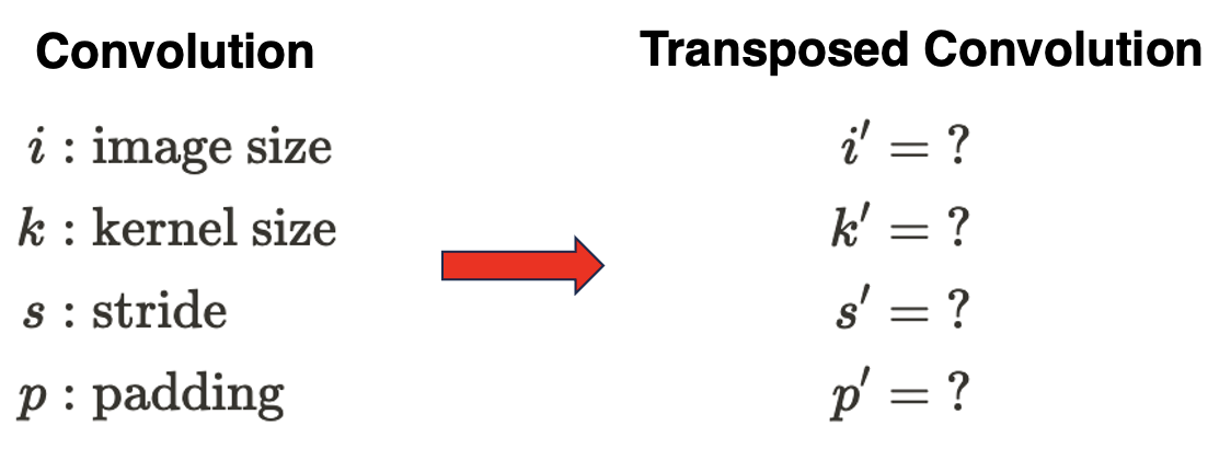
Here, $i^\prime = o$, $k^\prime = k$ always where $o = \lfloor \frac{i - k + 2p}{s} \rfloor + 1$.

Case 1: No padding and stride

For example, let $i = 4$, $k = 3$, $s = 1$ and $p = 0$. In this case, it is equivalent to the following convolution:

Hence, $i^\prime = \lfloor \frac{i - k + 2p}{s} \rfloor + 1$, $k^\prime = k$, $p^\prime = k - 1$ and $s^\prime = s$ in this case so that $o^\prime = i$.

We can observe the input of the transposed convolution is zero padded. One possible intuition to understand the logic of this is the connectivity pattern of convolution. The top leftmost pixel of input of convolution is connected to the top leftmost pixel of output only, and top rightmost pixel of input is directly connected to the top rightmost pixel of output only and similar connectivities to bottom corners. To maintain these connectivities in reconstruction (transposed convolution) too, we zero pad edges of input of transposed convolution to force pixels to hold down the fort in their pixels.

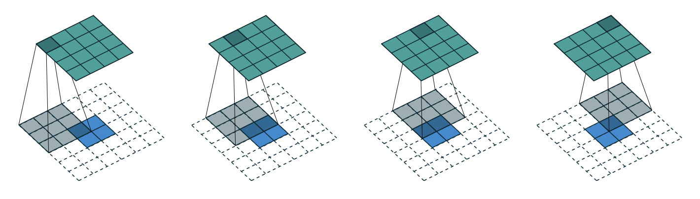
Case 2: Padded but no stride

Based on the connectivity interpretation of prior case, it is reasonable to think that the transpose of padded convolution is equivalent to convolving an input padded, but less. It is because zero padding in original convolution shifts the connectivities in edges to the center of output feature map, in order for avoiding information loss from the edges of the image while sliding window.

Here is an example of $i = 5$, $k = 4$, $p = 2$, and $s = 1$. Then $s^\prime = 1$ and $p^\prime = k - 1 - 2p$.

Hence, $o^\prime = \lfloor \frac{i - k + 2p}{s} \rfloor + 1 - k - 2p = i$

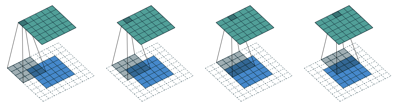
Case 3: No padding but non-unit strides

Let’s move on to non-unit strides cases. In the original convolution, the stride parameter $s$ indicates the speed of sliding of kernel through the input; in other words, it is related to the overlap of receptive fields. So, if $s$ is large, the connectivity between input and output feature map will be coarser. (On the other way, if $s$ is small the connectivity will be much finer) Hence, it is reasonable that if the kernel in convolution moved faster ( $s > 1$ ), then the kernel in corresponding transposed convolution should move faster too because the connection between input pixels and output pixels of transposed convolution will be rarely overlapped.

In the emulation with a direct convolution, we instead slow the kernel down to unit stride $s^prime = 1$ but instead dilate the input map of transposed convolution by inserting zeros between pixels. For instance, when $i = 5$, $k = 3$ and $s = 2$, zeros are inserted between input units, which makes the kernel move around at a slower pace than with unit strides.

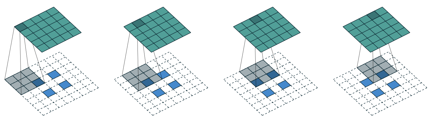
Generally, the stretched input is obtained by adding $s−1$ zeros between each input pixel. And, if we define $a = i - k + 2p \text{ mod } s$, equivalently $i - k + 2p = (i^\prime - 1)s + a$. Then, by setting $p^\prime = k - 1 - 2p + a$, the output size becomes $o^\prime = s(i^\prime - 1) + a + k - 2p = i$ clearly.

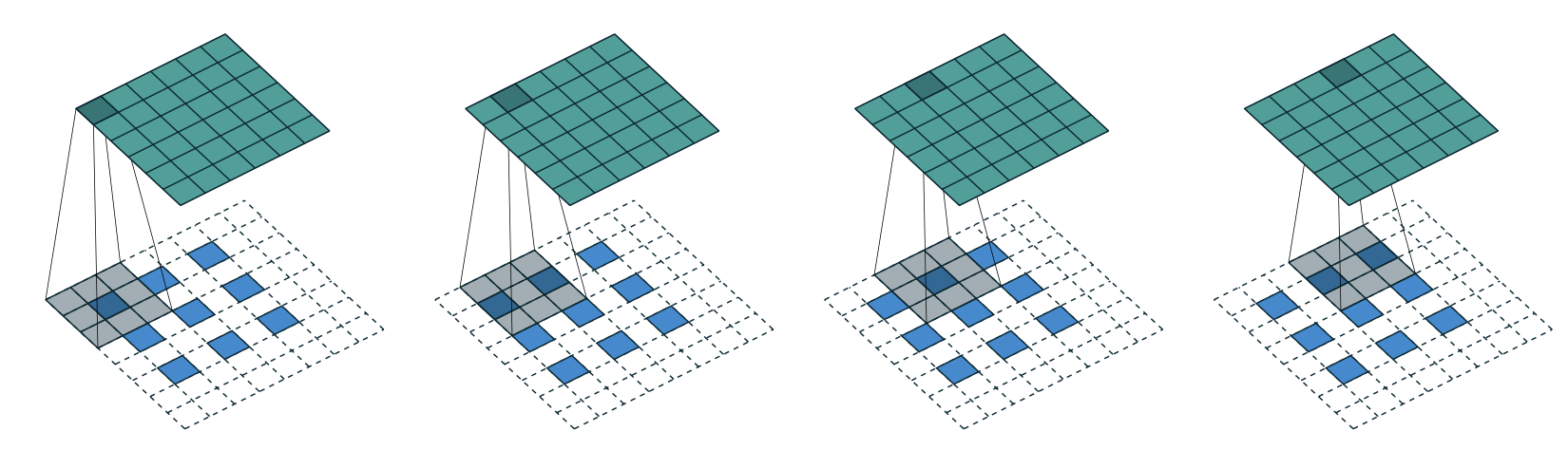
Case 4: Padded, and non-unit strides

Now, previous cases can be extended further to padded and non-unit strides case by combining each case. For example, for $i = 6$, $k = 3$, $s = 2$ and $p = 1$.

Two ways for emulation

Notably, it seems that transposed convolution can be emulated by two different ways. First one is via direct convolution as we saw above. And another is dot product, which is well explained in ProbML book by Kevin P. Murphy and CS231n lecture note. It is equivalent to padding the input image with $(h - 1, w - 1)$ $0$s (on the bottom right), where $(h, w)$ is the kernel size, then placing a weighted copy of the kernel on each one of the input locations, where the weight is the corresponding pixel value, and then adding up. Here is a visualization of this process.

But we don’t have to worry: two different approaches are exactly equivalent to each other if the kernel of a direct convolution is flipped. Here is a simple PyTorch notebook for comparisons.

It is just hard-coded, so it can’t be general implementation of transposed convolutions.

Transposed convolution in PyTorch and TensorFlow

When we apply convolution operation with non-unit stride, multiple combinations of kernel size, stride, and padding construct same output dimensions with different inputs. For example, $7 \times 7$ and $8 \times 8$ inputs would both return $3 \times 3$ output map if stride is $2$.

Hence, when we implement deconvolutional layers, it is not clear that which output shape of transposed convolution should return for these cases. In PyTorch and TensorFlow, transposed convolution module controls the output shape with additional argument called output_padding. Note that it doesn’t add any zero-padding to input or output.

Deconvolution v.s. Transposed Convolution

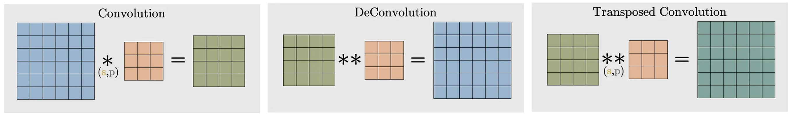
Note that transposed convolution is also sometimes called deconvolution, but this is an incorrect usage of the term: deconvolution is the process of “undoing” the effect of convolution with a known filter, such as a blur filter, to recover the original input, as illustrated in Figure 14.25.

So, why the confusion? Deconvolution is originally defined as stated on this Wikipedia page: https://en.wikipedia.org/wiki/Deconvolution. And as convolution does the exact opposite, so probably the upsampling of the feature map (transforming lower-dimensional feature maps into higher-dimensional feature maps) could be considered as a deconvolution operation. However, after reading several resources I conclude that there are several ways in which one can upsample the feature maps, like pixel shuffle (https://nico-curti.github.io/NumPyNet/NumPyNet/layers/pixelshuffle_layer.html) and transposed convolution (discussed earlier). Thus, all these operations do the same high-level thing but in a very different way (resulting in even different results).

Reference

[1] Dumoulin, Vincent, and Francesco Visin. “A guide to convolution arithmetic for deep learning.” arXiv preprint arXiv:1603.07285 (2016)
[2] Zhang, Aston, et al. “Dive into deep learning.”
[3] Enhancing CNN Models with Transposed Convolution Layers for Image Segmentation
[4] What is Transposed Convolutional Layer?
[5] What is the intuition behind transposed conv layers being able to upscale images?