
[DL] Knowledge Distillation
Knowledge Distillation
Knowledge distillation is model compression method where a small model is trained to replicate the cumbersome model (a pre-trained, larger model or ensemble of models). This training framework is sometimes referred to as “teacher-student learning”, where the large model is the teacher and the small model is the student.
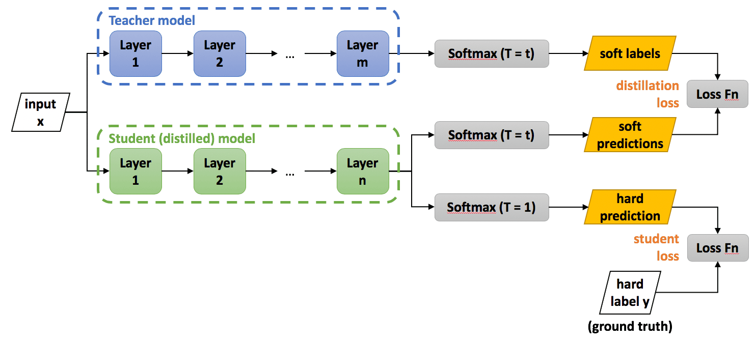
The knowledge distilation was first popularized by Hinton et al. 2015. They instantiated the knowledge of neural network by the neural response of the last output layer of the teacher model, which is termed as response-based knowledge. In image classification models, they typically produce class probabilities ($p_i$ for class $i$) by using a softmax:
\[p_i = \frac{\exp\left(\frac{z_i}{T}\right)}{\sum_{j} \exp\left(\frac{z_j}{T}\right)}\]where $T$ is a temperature factor. In many cases, for example in an easy dataset MNIST, the probability distribution has the correct class at a very high probability, with all other class probabilities very close to $0$. As such, it doesn’t provide much information beyond the ground truth labels already provided in the dataset. The softmax temperature can control the sharpness of the distribution, and it is possible to mitigate the issue.
Considering this probability output of the teacher model as soft target, the knowledge is distilled to the student model by minimizing the loss between the student’s soft prediction at a high temperature of $T = \tau$ and soft target, called distillation loss. Additionally, the student also self-studies the task by minimzing the loss between the student’s hard prediction at a temperature of $1$ and class label (hard target), called student loss. Accordingly, the total loss $\mathcal{L}$ for training can be rewritten as:
\[\begin{aligned} \mathcal{L} = \alpha \cdot \mathcal{L}_{\textrm{CE}}(y, \textrm{softmax}(\mathbf{z}_{\textrm{student}}; T=1)) + \beta \cdot \mathcal{L}_{\textrm{CE}}(\textrm{softmax}(\mathbf{z}_{\textrm{teacher}}; T=\tau), \textrm{softmax}(\mathbf{z}_{\textrm{student}}, T=\tau)) \end{aligned}\]
Knowledge Types
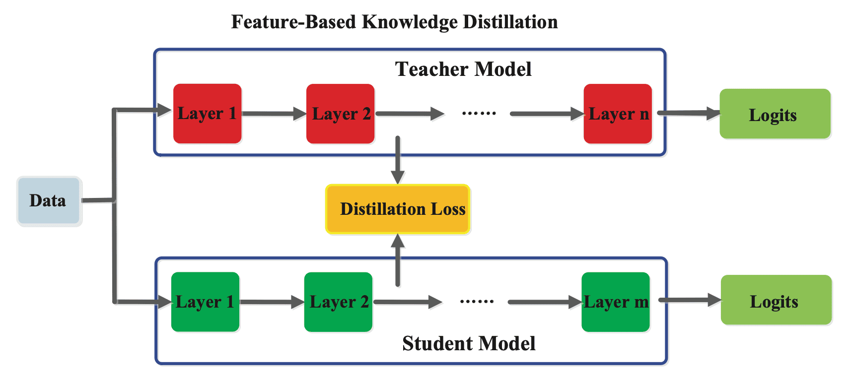
Feature-based Knowledge
While the concept of the response-based knowledge is straightforward and comprehensible, it becomes challenging to learn the intermediate representation and knowledge of the teacher model. Consequently, it falls short in harnessing the potential of deep neural networks to acquire hierarchical representations with increasing levels of abstraction. To mitigate the limitation, the knowledge used to supervise the training of the student model can be derived not only from the last layer but also from intermediate layers, i.e. feature maps.
FitNet
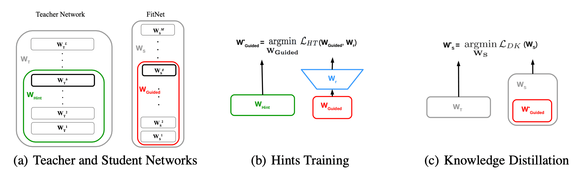
Fitnets (Romero et al. 2015) is the first approach that extend the knowledge distillation by using not only the outputs but also the intermediate representations learned by the teacher as hints to improve the training process and final performance of the student. Define a hint as the output of a teacher’s hidden layer responsible for guiding the student’s learning process. Let $h$-th hidden layer of the teacher model $\mathbf{T}$ and $g$-th hidden layer of the student model $\mathbf{S}$ be the hint layer and guided layer, respectively. Then, the loss function for hint-based training is written as
\[\begin{aligned} \mathcal{L}_{H T}\left(\mathbf{W}_{\text {Guided }}, \mathbf{W}_{\mathbf{r}}\right)=\frac{1}{2}\left\|\mathbf{T}_{1:h} \left(\mathbf{x} ; \mathbf{W}_{\text {Hint }}\right)-\mathbf{r} \left(\mathbf{S}_{1:g} \left(\mathbf{x} ; \mathbf{W}_{\text {Guided }}\right) ; \mathbf{W}_{\mathbf{r}}\right)\right\|^2, \end{aligned}\]where $f_{i:j}$ is the application of layers $i$ to $j$ of deep network $f$ inclusively, and \(\mathbf{W}_{\text {Hint }}\) and \(\mathbf{W}_{\text {Guided }}\) are the parameters of teacher/student network up to their respective hint/guided layers. Since the teacher model is usually wider than the student layer, a regressor $\mathbf{r}$ is added to the guided layer to match the output size. Then the fitnet (student model) is trained by jointly optimizing the hint training loss and knowledge distillation loss. The difference between them is illustrated in $\mathbf{Fig\ 3.}$
Attention Transfer
Inspired by Fitnet, a variety of other methods have been proposed to match the features indirectly. One of the most groundbreaking work of feature-based knowledge distillation is Attention Transfer proposed by Zagoruyko et al. 2017. The paper propose attention map as a mechanism of knowledge transfer from teacher network to student network, experimentally showing consistent improvement across a variety of datasets and convolutional neural network architectures.
The authors implicitly assumed that the absolute value of a hidden neuron activation $A \in \mathbb{R}^{C \times H \times W}$ can be used as an indication about the importance of that neuron w.r.t. the specific input. Accordingly, we can then construct a spatial attention map by computing statistics of these values across the channel dimension:
\[\begin{aligned} F_{\textrm{sum}} (A) & = \sum_{i=1}^C \lvert A_i \rvert \\ F_{\textrm{sum}}^p (A) & = \sum_{i=1}^C \lvert A_i \rvert^p \quad (p > 1) \\ F_{\textrm{max}} (A) & = \underset{1 \leq i \leq C}{\max} \lvert A_i \rvert^p \quad (p > 1) \end{aligned}\]The paper discovered that the aforementioned attention maps not only exhibit spatial correlation with predicted objects at the image level, but these correlations also tend to be more pronounced in networks with higher accuracy. Stronger networks demonstrate peaks in attention where weaker networks do not.
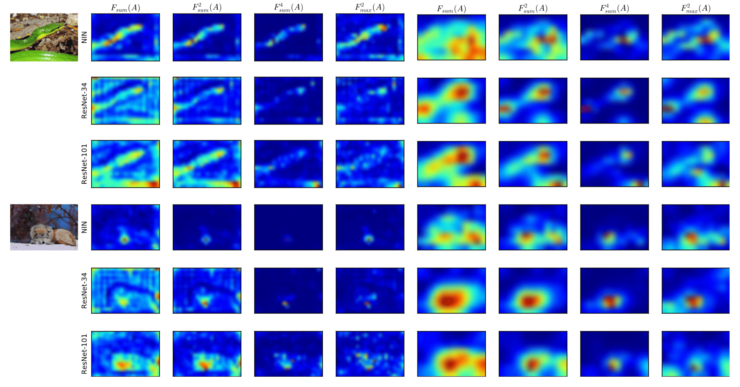
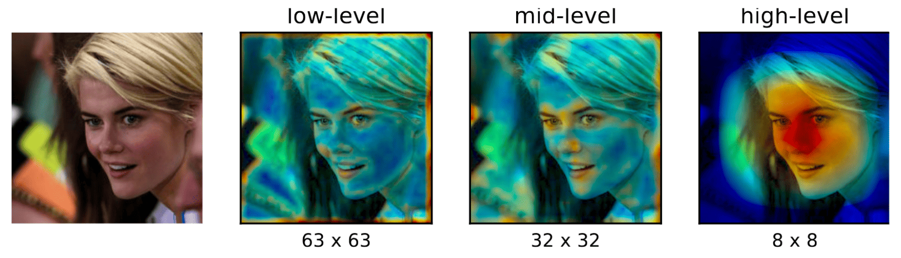
(Left) mid-level activations (Right) top-level pre-softmax activations (Zagoruyko et al. 2017)
Moreover, attention maps focus on different parts across different layers of the network. In the initial layers, neurons show highlighted activation for low-level gradient points. In the middle layers, the activation is more prominent for the most discriminative regions, such as eyes or wheels. Finally, in the top layers, the attention maps reflect entire objects. As an example, mid-level attention maps from a network trained for face recognition tend to have higher activations around eyes, nose, and lips, while top-level activation corresponds to the entire face.
the objective is to train a student network that not only makes correct predictions but also possesses attention maps that closely resemble those of the teacher. Transfer losses can be introduced with respect to attention maps computed across multiple layers. Without loss of generality, assume that transfer losses are placed between student and teacher attention maps of same spatial resolution. (If not, attention maps can be interpolated to match their shapes.) Let $S$, $T$ and $\mathbf{W}_S$, $\mathbf{W}_T$ denote student, teacher and their weights correspondingly. Let also $\mathcal{I}$ denote the indices of all teacher-student activation layer pairs for which we want to transfer attention maps. Then the total loss for training is defined as:
\[\begin{aligned} \mathcal{L} = \mathcal{L}_{\textrm{CE}} \left(\mathbf{x}; \mathbf{W}_S \right)+\frac{\beta}{2} \sum_{j \in \mathcal{I}}\lVert \frac{Q_S^j}{\lVert Q_S^j \rVert_2}-\frac{Q_T^j}{\lVert Q_T^j \rVert_2} \rVert_p \end{aligned}\]where $Q_S^j = \textrm{flatten}(F (A_S^j))$ and $Q_T^j = \textrm{flatten}(F (A_T^j ))$ are respectively the $j$-th pair of student and teacher attention maps in vectorized form, and $p$ refers to norm type (in the experiments they used $p = 2$).
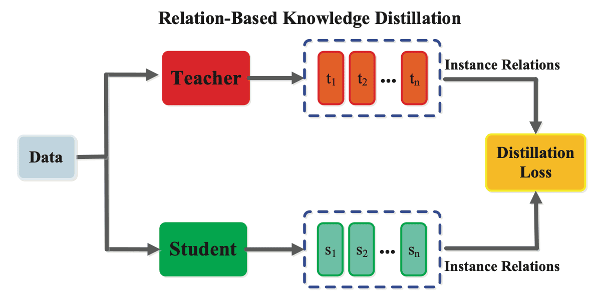
Relation-based Knowledge
Both response-based and feature-based knowledge exploit the outputs of last or intermediate layers in the teacher neural network. However, since there are many ways to solve the problem of generating the output from the input. In this context, mimicking the generated features or outputs of the teacher can still pose a challenging constraint for the student. In contrast, relation-based knowledge distillations exploit the relationships between different layers or data samples.
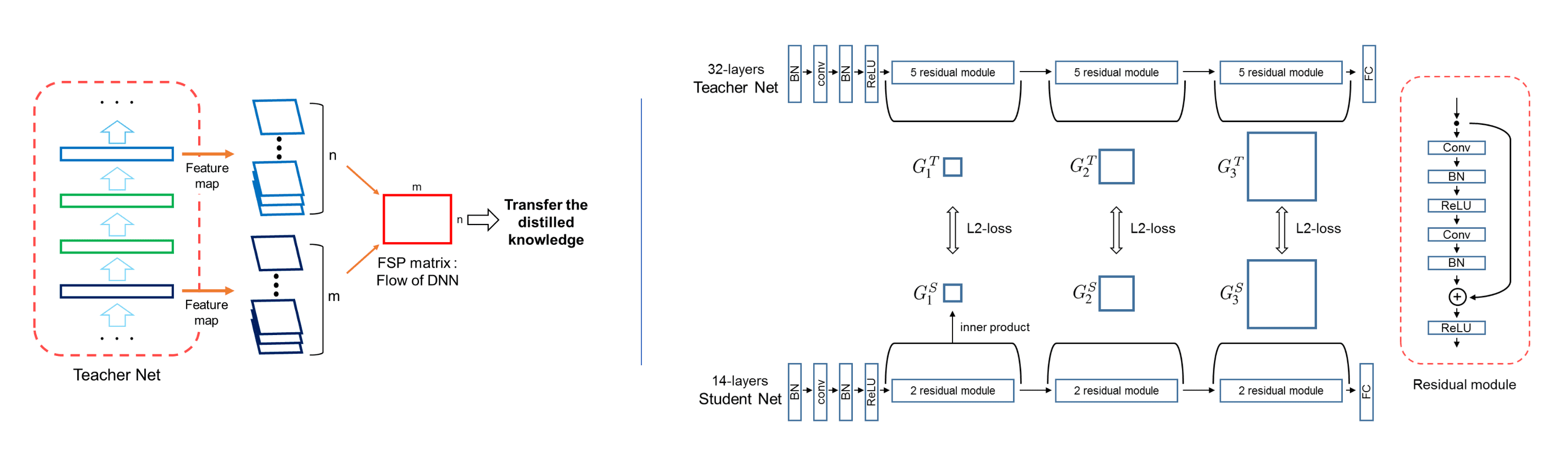
Flow of Solution Process
The first work on relation-based knowledge is flow of solution process (FSP) matrix, proposed by Yim et al. 2017. It is primarily inspired by the intuition that a genuine teacher imparts to a student the step-by-step approach for solving a problem. Because a DNN uses many layers sequentially to map from the input space to the output space, the flow of solving a problem can be defined as the relationship between features from two layers, represented by Gram matrix that contains the directionality between features. The FSP matrix $G \in \mathbb{R}^{m \times n}$ is generated by the features from two layers,$F^1 \in \mathbb{R}^{h \times w \times m}$ and $F^2 \in \mathbb{R}^{h \times w \times m}$:
\[G_{i, j}(\mathbf{x} ; \mathbf{W})=\sum_{s=1}^h \sum_{t=1}^w \frac{F_{s, t, i}^1(\mathbf{x} ; \mathbf{W}) \times F_{s, t, j}^2(\mathbf{x} ; \mathbf{W})}{h \times w}\]where $\mathbf{x}$ and $\mathbf{W}$ represent the input image and the parameters of the DNN. Then, for $n$ FSP matrices $G_i^T$ of teacher and $G_i^S$ of student, $i = 1, \cdots, n$, the squared $L_2$ norm between them is jointly optimized to distill the knowledge with the cost function from the original task:
\[L_{\textrm{FSP}}\left(\mathbf{W}_t, \mathbf{W}_s\right) = \frac{1}{N} \sum_{j = 1}^N \sum_{i=1}^n \lambda_i \times \| G_i^T \left(\mathbf{x}_j ; \mathbf{W}_t\right)-G_i^S\left(\mathbf{x}_j ; \mathbf{W}_s\right) \|_2^2\]
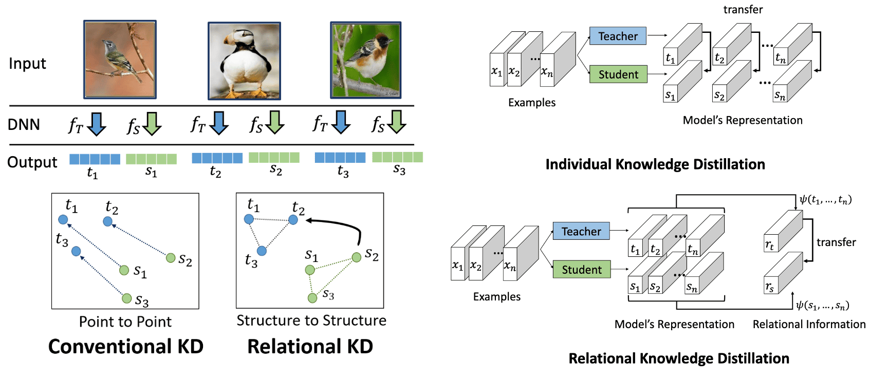
Relational Knowledge Distillation
Thus far, traditional knowledge transfer methods that we have discussed involve the individual knowledge derived from the individual data example. However, the distilled knowledge can encompass not only feature information but also the mutual relations between data samples. This forms the core principle of Relational Knowledge Distillation (RKD) proposed by Park et al. 2019 that what constitutes the knowledge is better encapsulated by the relationships among learned representations rather than individual instances.
Given a teacher model $T$ and a student model $S$, let $f_T$ and $f_S$ be functions of the teacher and the student, respectively. Denote by $\mathcal{X}^N$ a set of $N$-tuples of distinct data examples, e.g., \(\mathcal{X}^2 = \{ (\mathbf{x}_i, \mathbf{x}_j ) \vert i \neq j \}\) and \(\mathcal{X}^3 = \{ (\mathbf{x}_i, \mathbf{x}_j, \mathbf{x}_k ) \vert i \neq j \neq k \}\). Conventional KD methods can commonly be expressed as minimizing the following objective function:
\[\mathcal{L}_{\textrm{IKD}} = \sum_{\mathbf{x}_i \in \mathcal{X}} \mathcal{L} (f_T (\mathbf{x}_i), f_S (\mathbf{x}_i))\]For notational simplicity, let us define \(\mathbf{t}_i = f_T (\mathbf{x}_i)\) and \(\mathbf{s}_i = f_S (\mathbf{x}_i)\). The objective for RKD aims at transferring structural knowledge using mutual relations of data examples in the teacher’s output representation, using a relational potential $\psi$ for each $n$-tuple of data examples:
\[\mathcal{L}_{\textrm{RKD}} = \sum_{(\mathbf{x}_1, \cdots, \mathbf{x}_n) \in \mathcal{X}^N} \mathcal{L} (\psi(\mathbf{t}_1, \cdots, \mathbf{t}_n) ,\psi (\mathbf{s}_1, \cdots, \mathbf{s}_n ))\]In this perspective, relational knowledge distillation is the generalized version of individual knowledge distillation. And the effectiveness and efficiency of RKD relies on the choice of the potential function $\psi$. Park et al. 2019 propose two simple yet effective pairwise and ternary relations: distance-wise and angle-wise losses.
\[\begin{aligned} \psi_D (\mathbf{t}_i, \mathbf{t}_j) = \frac{1}{\mu} \lVert \mathbf{t}_i - \mathbf{t}_j \rVert_2 \text{ where } \mu = \frac{1}{\lvert \mathcal{X}^2 \rvert} \sum_{(\mathbf{x}_i, \mathbf{x}_j) \in \mathcal{X}^2} \lVert \mathbf{t}_i - \mathbf{t}_j \rVert_2 \end{aligned} \\ \begin{aligned} & \psi_{\mathrm{A}}\left(\mathbf{t}_i, \mathbf{t}_j, \mathbf{t}_k\right)=\cos \angle \mathbf{t}_i \mathbf{t}_j \mathbf{t}_k=\left\langle\mathbf{e}^{i j}, \mathbf{e}^{k j}\right\rangle \\ & \text { where } \quad \mathbf{e}^{i j}=\frac{\mathbf{t}_i-\mathbf{t}_j}{\left\|\mathbf{t}_i-\mathbf{t}_j\right\|_2}, \mathbf{e}^{k j}=\frac{\mathbf{t}_k-\mathbf{t}_j}{\left\|\mathbf{t}_k-\mathbf{t}_j\right\|_2} . \end{aligned}\]
Distillation Strategies
The learning schemes of knowledge distillation can be directly categorized into three main types based on whether the teacher model is updated simultaneously with the student model: offline distillation, online distillation, and self-distillation. Most of knowledge distillation methods (including the methods we’ve discussed thus far) fall into offline, i.e. require the pre-trained teacher model (hence two-phase training) and employ one-way knowledge transfer. In spite of its simplicity, the main downside is that large networks are harder to train and find the right parameters for the task.
Online Distillation
To overcome the limitation of offline distillation, a variety of works proposed different methodologies for online distillation, including mutual learning and co-distillation.
Deep Mutual Learning
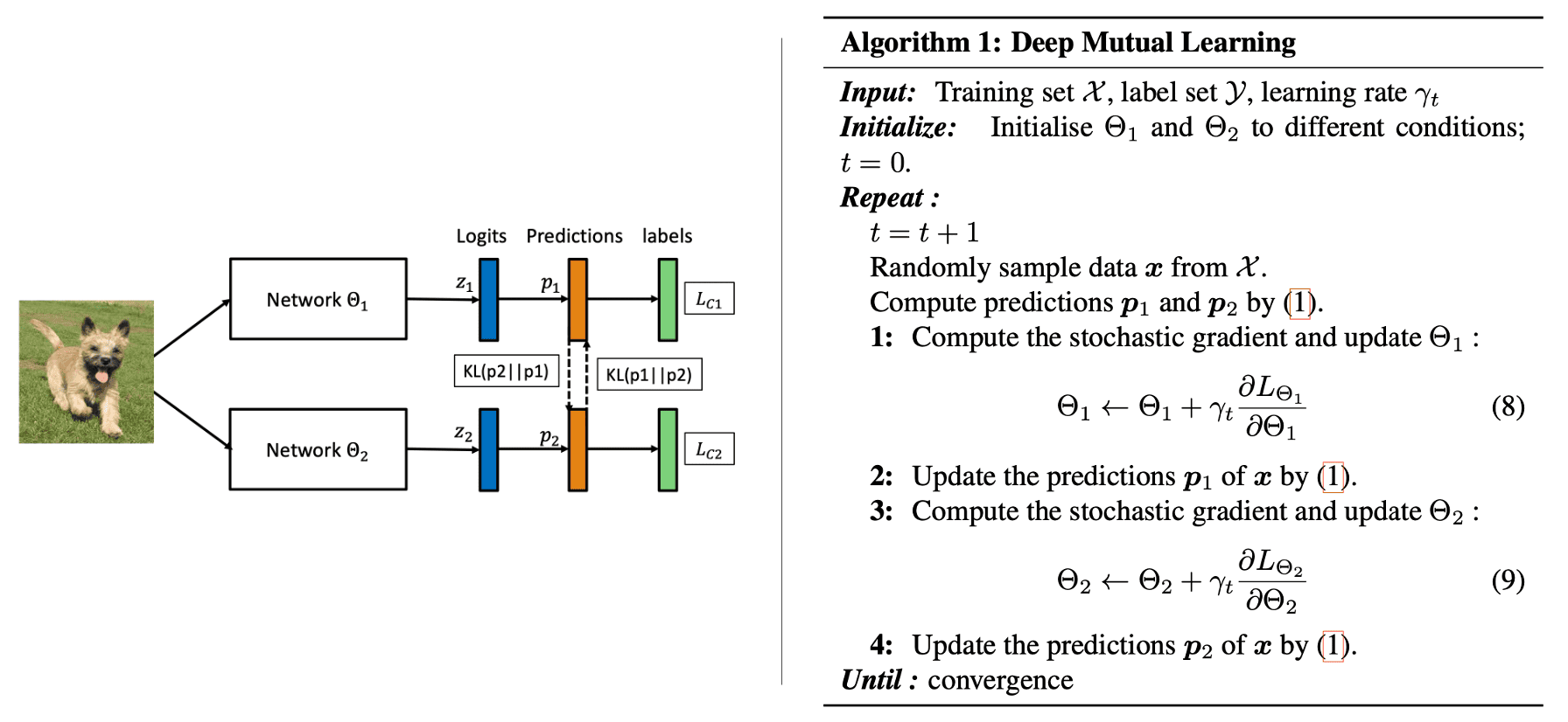
Deep Mutual Learning (Zhang et al. 2018) is one of pioneering works in online distillation. In deep mutual learning, a pool of $K$ untrained students simultaneously learn to solve the task together. Each student is trained with two losses: a supervised learning loss, and a mimicry loss. Given $N$ samples \(\mathcal{X} = \{ \boldsymbol{x}_i \}_{i=1}^N\) from $M$-label set as \(Y = \{y_i\}_{i=1}^N\) with \(y_i \in \{1, 2, \cdots, M \}\). Then, a conventional supervised learning loss for softmax classifier network $f_{\boldsymbol{\Theta}_k}$ ($k = 1, \cdots, K$) is defined as the cross entropy error:
\[\begin{aligned} \mathcal{L}_{\textrm{CE}, k} = - \sum_{i=1}^N \sum_{m=1}^M \mathbb{I}(y_i, m) \cdot \log f_{\boldsymbol{\Theta}_k} (\boldsymbol{x}_i) \end{aligned}\]Some insights into a group of students can be gained by considering the following. Each student is primarily directed by a supervised learning loss, their performance generally increases and they cannot drift arbitrarily into wrong way. But since each network starts from a different initial condition, they learn different representations, and this will provide the extra information in distillation. And a mimicry loss aligns each student’s class posterior with the class probabilities of other students:
\[\begin{aligned} \mathcal{L}_{\textrm{mimic}, k} & = \frac{1}{K-1} \sum_{\ell = 1, \ell \neq k}^K \mathrm{KL}(\mathbf{p}_\ell \Vert \mathbf{p}_k) \\ & = \frac{1}{K-1} \sum_{\ell = 1, \ell \neq k}^K \sum_{i=1}^N \sum_{m=1}^M f_{\boldsymbol{\Theta}_\ell}^m (\boldsymbol{x}_i) \log \frac{f_{\boldsymbol{\Theta}_\ell}^m (\boldsymbol{x}_i)}{f_{\boldsymbol{\Theta}_k}^m (\boldsymbol{x}_i)} \end{aligned}\]where the coefficient $1/(K-1)$ is added in order to make sure that the training is mainly directed by supervised learning of the true labels. Intuitively, matching the other most likely classes for each training student according to their peers helps them to converge to a more robust minima with better generalization.
Co-distillation
Anil et al. ICLR 2018 proposed another methodology of online distillation called co-distillation, to train large-scale distributed neural network. $\mathbf{Fig\ 10.}$ shows the general framework of codistillation. Co-distillation in parallel trains multiple models with the same architectures, where each model is trained by transferring knowledge from the other models.
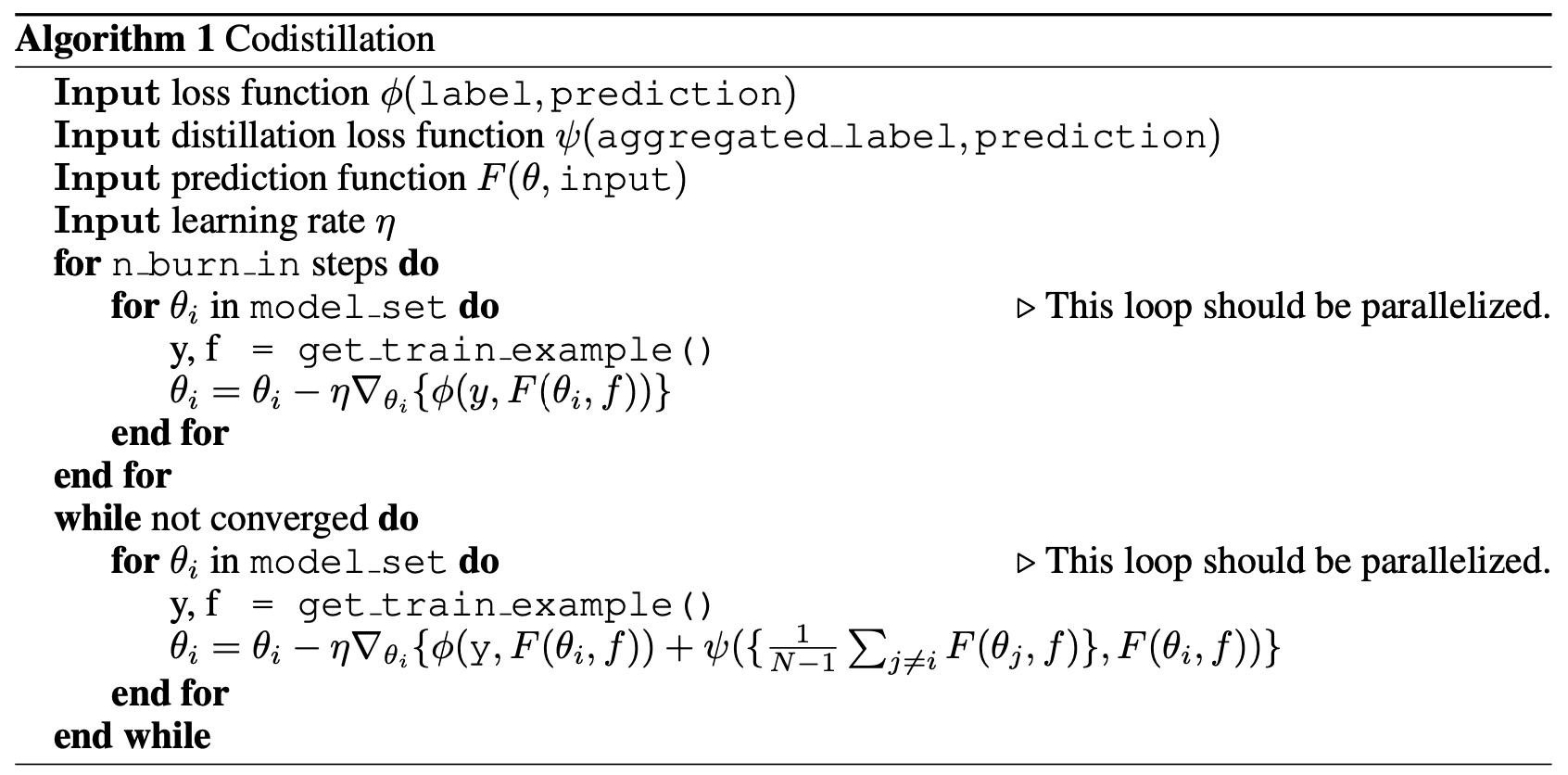
The distillation loss term $\psi$ can be any form of distillation, e.g. the squared error between the logits of the models, the KL divergence between the predictive distributions, or some other measure of agreement between the model predictions. In the beginning of training, the distillation term in the loss may not be very beneficial or may even hamper the optimization. To maintain model diversity longer and simplify the loss function schedule, the distillation term is only activated in the loss function once training has gained momentum.
Self-Distillation
Thus far, teacher models and student models operate independently, and knowledge transfer occurs among different models. However, the drawback is low efficiency in transfer, resulting in student models insufficiently leveraging all knowledge from teacher and exhibiting inferior performance than teacher. Another challenge lies in the design and training of proper teacher models. It demands considerable effort and experiments to identify the optimal architecture for teacher models, which takes a relatively long time.
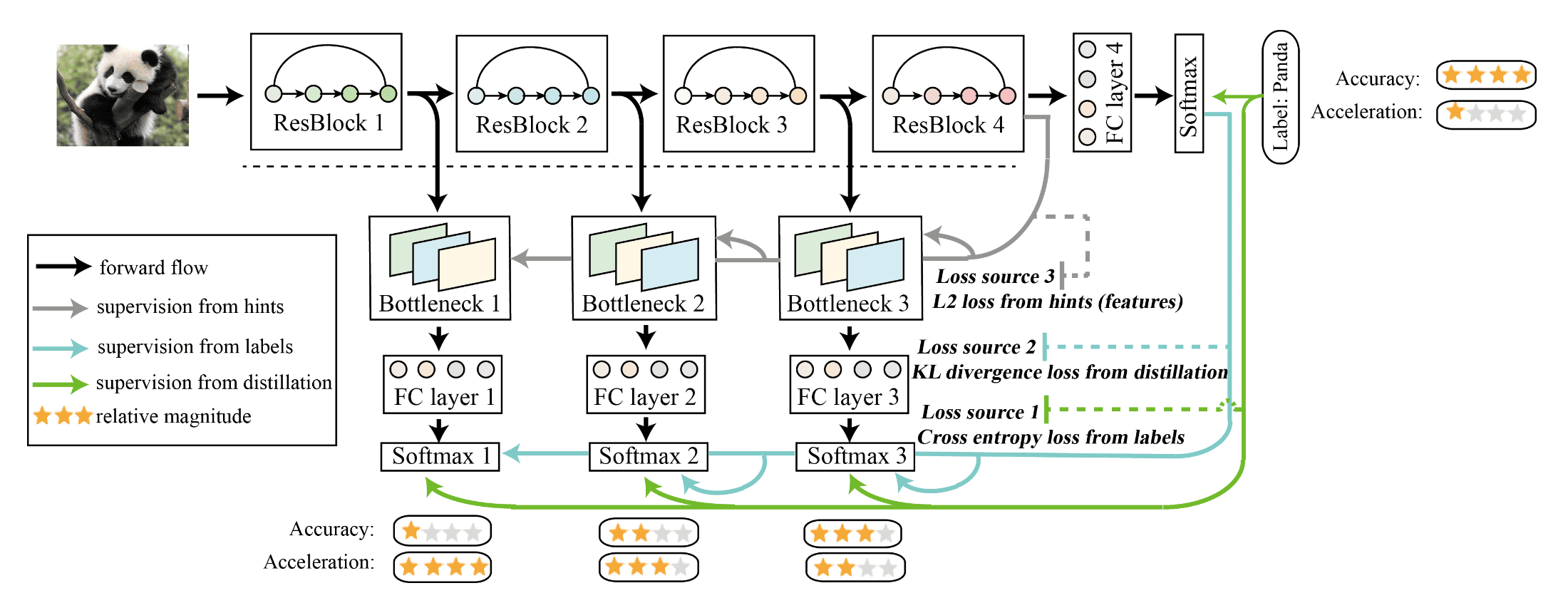
In self-distillation, the same networks are used for the teacher and the student models, which can be viewed as a special case of online distillation. It is first proposed by Zhang et al. CVPR 2019 for convolutional neural networks. The target convolutional neural network is divided into several shallow sections according to its depth and original structure. (As an example, ResNet50 can be divided into 4 sections according to ResBlocks.) Then, a classifier is established for each section, incorporating a bottleneck layer and a fully connected layer. The bottleneck layer is added here in order to mitigate the impacts between each shallow classifier, and to add $L_2$ loss from hints. And these classifiers are exclusively employed during training and can be omitted during inference.
Given $N$ samples \(X = \{ \mathbf{x}_i \}_{i=1}^N\) from $M$ classes and the corresponding label set as \(Y = \{y_i \vert y_i \in \{ 1, 2, \cdots, M \}\}_{i=1}^M\), denote classifiers in the neural network as \(\Theta = \{ \theta_{i/C} \}_{i=1}^C\) where $C$ denotes the number of classifiers in convolutional neural networks. A softmax layer is set after each classifier:
\[\begin{aligned} \mathbf{q}_i^c=\frac{\exp \left(\mathbf{z}_i^c / \tau \right)}{\Sigma_j^c \exp \left(\mathbf{z}_j^c / \tau \right)} \end{aligned}\]where $\mathbf{z}$ is the output after fully connected layers and \(\mathbf{q}_i^c \in \mathbb{R}^M\) is the $i$-th class probability of classifier $\theta_{c/C}$. While in training period, knowledge (features, logits) from the deeper sections of the network is distilled into its shallow sections and therefore there are 3 kinds of losses for optimization. (Two hyper-parameters $\alpha$ and $\lambda$ are used to balance them.)
- Cross entropy loss from labels
For the softmax layer’s output of classifier $\theta_{j/C}$, $\mathbf{q}^j$, $$ (1 - \alpha) \cdot \mathcal{L}_{\textrm{CE}} (\mathbf{q}^j, \mathbf{y}) $$ - KL divergence loss under teacher’s guidance.
$$ \begin{aligned} \alpha \cdot \textrm{KL} (\mathbf{q}^j \Vert \mathbf{q}^C) \end{aligned} $$ - $L_2$ loss from hints (features)
It is computed by $L_2$ loss between features maps of the deepest classifier and each shallow classifier. As a result, the inexplicit knowledge in feature maps is introduced to each shallow classifier’s bottleneck layer. $$ \begin{aligned} \lambda \cdot \lVert F_i - F_C \rVert_2^2 \end{aligned} $$ where $F_i$ and $F_C$ denote features in the classifier $\theta_i$ and features in the deepest classifier $\theta_C$ respectively.
Note that $\lambda$ and $\alpha$ for the deepest classifier are $0$, which means the deepest classifier’s supervision just comes from labels. Hence, conceptually, all the shallow sections with corresponding classifiers can be regarded as students and trained via via distillation from the deepest section, which can be viewed as the teacher.
Reference
[1] Gou et al., “Knowledge Distillation: A Survey”, IJCV 2021
[2] Hinton et al. “Distilling the knowledge in a neural network”, arXiv:1503.02531 2015
[3] “Knowledge Distillation”, Intel Labs
[4] Romero et al., “FitNets: Hints for Thin Deep Nets”, ICLR 2015
[5] Zagoruyko et al., “Paying More Attention to Attention: Improving the Performance of Convolutional Neural Networks via Attention Transfer”, ICLR 2017
[6] Yim et al., “A Gift from Knowledge Distillation: Fast Optimization, Network Minimization and Transfer Learning”, CVPR 2017
[7] Park et al., “Relational Knowledge Distillation”, CVPR 2019
[8] Zhang et al., “Deep Mutual Learning”, CVPR 2018
[9] Anil et al., “Large scale distributed neural network training through online distillation”, ICLR 2018
[10] Zhang et al., “Be Your Own Teacher: Improve the Performance of Convolutional Neural Networks via Self Distillation”, CVPR 2019
Leave a comment