[DL] Natural Gradient

The stochastic gradient method is widely adopted in the field of optimization. However, in many cases, the space of deep neural networks is not Euclidean but possesses a Riemannian metric structure, rendering the ordinary gradient fails to provide the steepest direction of the function. The natural gradient, on the other hand, extends beyond the conventional gradient, incorporating the curvature of the function being optimized. Hence when applied to optimization problems, natural gradient descent can markedly improve convergence speed compared to vanilla gradient descent.

Motivation

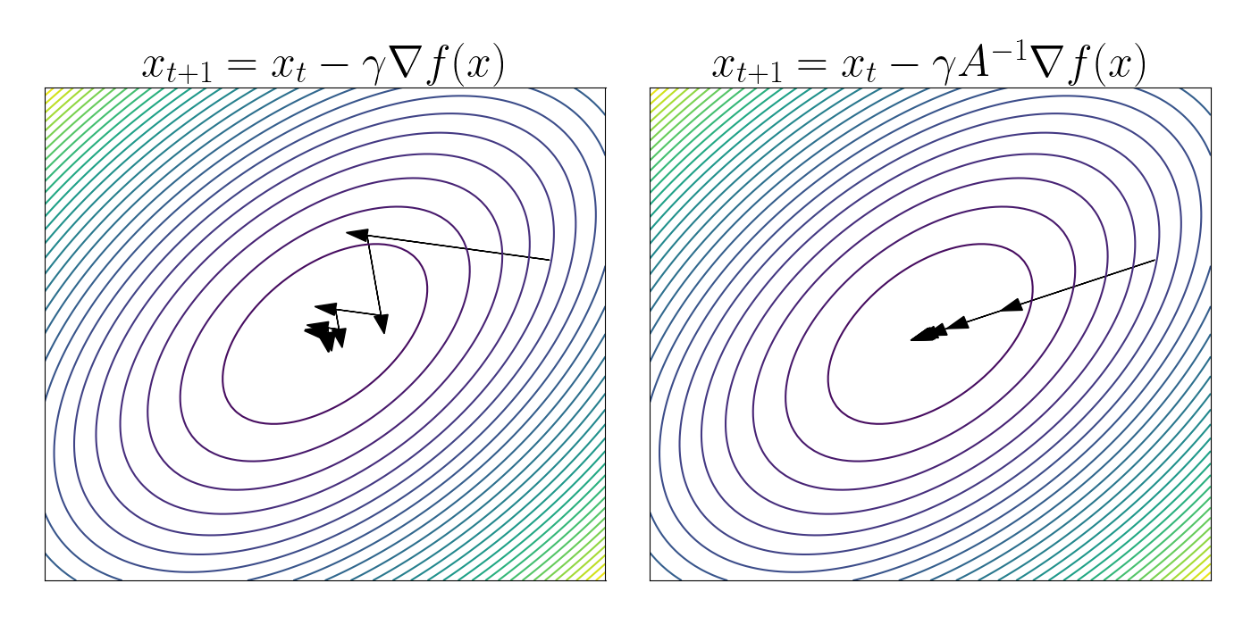
Stochastic Gradient Descent (SGD) tends to oscillate in regions of high curvature while progressing slowly in areas of low curvature. This behavior stems from the fact that when training neural networks, we optimize over a complex manifold of functions. Transforming this manifold into an orthonormal coordinate system distorts distances, contributing to the uneven progress of SGD in different directions.

$\mathbf{Fig\ 1.}$ (Left) SGD that doesn't compensate the curvature (Right) Natural Gradient Descent (Andy Jones)

Hence, we necessitate the optimization algorithm that remains invariant to the coordinate system. For intuition, consider the task of finding a minimizer $x^\star$ of function $f(x)$, where $x$ is measured in $m^2$ and the value of $f$ is measured in $m$. In typical gradient descent with learning rate $\alpha$, our estimation of $x^\star$ is iteratively updated as

\[x \leftarrow x - \alpha \frac{df}{dx}\]

However, $df/dx$ has units $1/m$. Therefore, we are adding quantities with units $m^2$ and $m^{-1}$, which is nonsensical. This discrepancy is the reason why gradient descent encounters issues with poorly scaled data.

Preliminary: Fisher Information

Let $p_{\boldsymbol{\theta}} (x)$ be the probability density function. In statistics, the gradient of log-likelihood $\nabla_{\boldsymbol{\theta}} \log p_\boldsymbol{\theta} (x)$ is called score, and the covariance of score

\[\mathbf{F} (\boldsymbol{\theta}) = \mathbb{E}_{x \sim p_{\boldsymbol{\theta}} (\cdot)} \left[ \frac{\partial \log p_\boldsymbol{\theta} (x)}{\partial \boldsymbol{\theta}} \frac{\partial \log p_\boldsymbol{\theta} (x)}{\partial \boldsymbol{\theta}}^\top \right]\]

is called Fisher information.

Negative Expectation of Hessian

We claim that \(\mathbf{F}(\boldsymbol{\theta})=−\mathbb{E}_{x \sim p_\boldsymbol{\theta}(x)}[\mathbb{H}(\log p_\boldsymbol{\theta}(x))]\). In other words, the Fisher information matrix $\mathbf{F}(\boldsymbol{\theta})$ contains the information about the curvature in our likelihood-based loss function. Note that

\[\begin{aligned} \mathbb{H}(\text{log } p_\boldsymbol{\theta} (x)) & = \nabla_\boldsymbol{\theta} \frac{\nabla_\boldsymbol{\theta} p_\boldsymbol{\theta} (x)}{p_\boldsymbol{\theta} (x)} \\ & = \frac{\mathbb{H} ( p_\boldsymbol{\theta} (x) )}{p_\boldsymbol{\theta} (x)} - \left( \frac{\nabla_\boldsymbol{\theta} p_\boldsymbol{\theta} (x)}{p_\boldsymbol{\theta} (x)} \right) \left( \frac{\nabla_\boldsymbol{\theta} p_\boldsymbol{\theta} (x)}{p_\boldsymbol{\theta} (x)} \right)^\top \end{aligned}\]

By taking the expectation,

\[\begin{aligned} \mathbb{E}_{x \sim p_\boldsymbol{\theta}(x)} \left[ \mathbb{H}(\text{log } p_\boldsymbol{\theta} (x))\right] & = \mathbb{E}_{x \sim p_\boldsymbol{\theta} (x)}\left[\frac{\mathbb{H} ( p_\boldsymbol{\theta} (x) )}{p_\boldsymbol{\theta} (x)}\right] - \mathbf{F}(\boldsymbol{\theta}) \\ & = \int \frac{\mathbb{H} (p_\boldsymbol{\theta} (x))}{p_\boldsymbol{\theta} (x)} p_\boldsymbol{\theta} (x) \cdot dx - \mathbf{F}(\boldsymbol{\theta}) \\ & = \mathbb{H} \left( \int p_\boldsymbol{\theta} (x) dx \right) - \mathbf{F}(\boldsymbol{\theta} ) \\ & = - \mathbf{F}(\boldsymbol{\theta}) \end{aligned}\]

Connection with KL divergence

KL divergence can be connected to a Riemannian metric called Fisher information metric:

\[\begin{aligned} \textrm{KL}(p_\boldsymbol{\theta} (x) \Vert p_{\boldsymbol{\theta}^\prime} (x)) \approx \frac{1}{2} \delta^{\top} \mathbf{F}(\boldsymbol{\theta}) \delta \end{aligned}\]

for small $\delta = \boldsymbol{\theta} - \boldsymbol{\theta}^\prime$. This is obtained by 2nd order Taylor approximation at $\boldsymbol{\theta}$:

\[\begin{aligned} \textrm{KL}(p_\boldsymbol{\theta} (x) \Vert p_{\boldsymbol{\theta}^\prime} (x)) & \approx \textrm{KL}(p_\boldsymbol{\theta} (x) \Vert p_{\boldsymbol{\theta}} (x)) + (\left. \nabla_{\boldsymbol{\theta}} \textrm{KL}(p_\boldsymbol{\theta} (x) \Vert p_{\boldsymbol{\theta}^\prime} (x)) \right|_{\boldsymbol{\theta}^\prime = \boldsymbol{\theta}})^\top \delta + \frac{1}{2} \delta^\top \mathbf{F}(\boldsymbol{\theta}) \delta \\ & = (\left. \nabla_{\boldsymbol{\theta}} \textrm{KL}(p_\boldsymbol{\theta} (x) \Vert p_{\boldsymbol{\theta}^\prime} (x)) \right|_{\boldsymbol{\theta} = \boldsymbol{\theta}^\prime})^\top \delta + \frac{1}{2} \delta^\top \mathbf{F}(\boldsymbol{\theta}) \delta \end{aligned}\]

From the fact that the expectation of score function $\nabla_{\boldsymbol{\theta}} \text{ log } p_\boldsymbol{\theta} (x)$ is zero:

\[\begin{aligned} \mathbb{E}_{x \sim p_\boldsymbol{\theta}(x)} \left[ \nabla_{\boldsymbol{\theta}} \text{ log } p_\boldsymbol{\theta} (x) \right] & = \int \left( \nabla_{\boldsymbol{\theta}} \text{ log } p_\boldsymbol{\theta}(x) \right) \cdot p_\boldsymbol{\theta}(x) \cdot dx \\ & = \int \nabla_{\boldsymbol{\theta}} p_\boldsymbol{\theta}(x) \cdot dx \\ & = \nabla_{\boldsymbol{\theta}} \int p_\boldsymbol{\theta}(x) \cdot dx = 0 \end{aligned}\]

done.

Why is it called “Information”?

“Information” is a conceptual construct that can be measured in various ways. Shannon’s method involves compressing data to its utmost and then tallying the number of bits required in the most condensed form. In contrast, Fisher’s approach diverges significantly and aligns more closely with laymen’s intuitive understanding. For instance, if presented with data on rat death rates in China and asked to estimate the population of Cuba based on this data, one would discern that the data offers no pertinent information about the quantity to be estimated.

In a broader sense, information can be quantified as follows: attempt your “best” to estimate the quantity of interest based on the available data, and assess how “well” you have performed. Maximum likelihood estimation (MLE) often serves as the natural choice for determining the “best” estimation, while considering the variance of the MLE provides a metric for assessing performance. A smaller variance corresponds to more “information.” Consequently, considering the reciprocal of the variance yields a measure of information. As the sample size grows large, the limiting behavior of this measure converges to Fisher information.

Also, see [5] for why the gradient of log-likelihood is called “score”

Steepest Descent

Let’s consider the problem finding the steepest descent direction of a function $f(\boldsymbol{x})$ at $\boldsymbol{x}$. Formally, the solution of this problem is defined by the vector $d\boldsymbol{x}$ that minimizes $f(\boldsymbol{x} + d\boldsymbol{x})$ where $\lVert d\boldsymbol{x} \rVert$ has a fixed length $\varepsilon$:

\[d\boldsymbol{x} = \underset{\lVert d\boldsymbol{x} \rVert = \varepsilon}{\textrm{arg min }} f(\boldsymbol{x} + d\boldsymbol{x})\]

A crucial observation here is that the metric $\lVert \cdot \rVert$ of step lengths hinges on the geometric characteristics of the problem. Indeed, the typical gradient descent is the solution of the optimization problem if we assume Euclidean metric ($L_2$ distance) for $\lVert \cdot \rVert$.

Note that gradient defines a linear approximation to a function, $f(\boldsymbol{x} + d\boldsymbol{x}) \approx f(\boldsymbol{x}) + \nabla f(\boldsymbol{x})^\top d\boldsymbol{x}$. We put $d\boldsymbol{x} = \varepsilon \boldsymbol{z}$, and search for the $\boldsymbol{z}$ that minimizes $f(\boldsymbol{x} + d\boldsymbol{x}) \approx f(\boldsymbol{x}) + \nabla f(\boldsymbol{x})^\top (\varepsilon \boldsymbol{z})$ under the constraint $\lVert \boldsymbol{z} \rVert = 1$. By the Lagrange multiplier method, we have

\[\begin{aligned} & \frac{\partial}{\partial z_i} \left[ f(\boldsymbol{x} + \boldsymbol{z}) - \lambda \lVert \boldsymbol{z} \rVert \right] \\ \approx \; & \frac{\partial}{\partial z_i} \left[ f (\boldsymbol{x}) + \nabla f(\boldsymbol{x})^\top \boldsymbol{z} - \lambda \lVert \boldsymbol{z} \rVert \right] = 0 \end{aligned}\]

which gives $\nabla f(\boldsymbol{x}) = \lambda \boldsymbol{z}$ where the Lagrange multiplier $\lambda$ is determined from the constraint.

Natural Gradient

Amari et al. 1998 showed that the steepest descent direction in general depends on the Riemannian metric tensor of the parameter space. Let \(S = \{ \boldsymbol{x} \in \mathbb{R}^n\}\) be a parameter space on which a function $f(\boldsymbol{x})$ is defined. When $S$ is a Euclidean space with an orthonormal coordinate system $\boldsymbol{x}$, the squared length of a small incremental vector $d\boldsymbol{x}$ is given by

\[\lVert d\boldsymbol{x} \rVert^2 = \sum_{j=1}^n d\boldsymbol{x}_j^2\]

When $S$ is a curved manifold, there is no orthonormal linear coordinates. Here, we can obtain a generalized version of the Pythagorean theorem for a Riemannian manifold:

\[\lVert d\boldsymbol{x} \rVert^2 = \sum_{i, j} g_{ij} (\boldsymbol{x}) d\boldsymbol{x}_i d\boldsymbol{x}_j = \boldsymbol{x}^\top \mathbf{G} \boldsymbol{x}\]

The $n \times n$ matrix $\mathbf{G} = (g_{ij})$ is called the Riemannian metric tensor, and it depends in general on coordinate system $\boldsymbol{x}$. Note that $g_{ij} = \delta_{ij}$, i.e. $\mathbf{G} = \mathbb{I}_{n \times n}$ in the Euclidean orthonormal case.

Amari et al. 1998 proved that the steepest descent direction in a space with metric tensor $\mathbf{G}$ is given by

\[\tilde{\nabla} f(\boldsymbol{x}) = \mathbf{G}^{-1}(\boldsymbol{x}) \nabla f(\boldsymbol{x}).\]

and termed this gradient as natural gradient in the Riemannian space. The proof is identical to the previous section; by the Lagrange multiplier method, the optimization problem is reduced to

\[\begin{aligned} & \frac{\partial}{\partial z_i} \left[ f(\boldsymbol{x} + \boldsymbol{z}) - \lambda \boldsymbol{z}^\top \mathbf{G} \boldsymbol{z} \right] \\ \approx \; & \frac{\partial}{\partial z_i} \left[ f (\boldsymbol{x}) + \nabla f(\boldsymbol{x})^\top \boldsymbol{z} - \lambda \boldsymbol{z}^\top \mathbf{G} \boldsymbol{z} \right] = 0 \end{aligned}\]

which gives $\nabla f(\boldsymbol{x}) = 2 \lambda \mathbf{G} \boldsymbol{z}$, equivalently

\[\boldsymbol{z}^\star = \frac{1}{2\lambda} \mathbf{G}^{-1} \nabla f(\boldsymbol{x})\]

where the Lagrange multiplier $\lambda$ is determined from the constraint.

$\color{blue}{\mathbf{Definition.}}$ Natural Gradient
We call $$ \tilde{\nabla} f(\boldsymbol{x}) = \mathbf{G}^{-1}(\boldsymbol{x}) \nabla f(\boldsymbol{x}) $$ the natural gradient of $f$ in the Riemannian space that represents the steepest descent direction of $f$.

Natural Gradient Learning of Probability Density Function

In the scenario of optimizing the parameterized probabilistic model $p_\boldsymbol{\theta}$ by $\boldsymbol{\theta}$, i.e. the optimization variables parameterize the probability distribution, the natural metric is KL divergence:

\[\lVert \boldsymbol{\theta}_{t+1} - \boldsymbol{\theta}_t \rVert = \textrm{KL} (p_{\boldsymbol{\theta}_{t+1}} \Vert p_{\boldsymbol{\theta}_t})\]

From the preliminary, it is equivalent to

\[\textrm{KL} (p_{\boldsymbol{\theta}_{t+1}} \Vert p_{\boldsymbol{\theta}_t}) = \frac{1}{2} d\boldsymbol{\theta}^\top \mathbf{F}(\boldsymbol{\theta}_t) d\boldsymbol{\theta}\]

where $\mathbf{F}$ is the Fisher information matrix. Hence, in the training of probabilistic model, our natural gradient descent is defined by

\[\begin{aligned} \boldsymbol{\theta}_{t+1} & \leftarrow \boldsymbol{\theta}_t - \alpha \tilde{\nabla} p_{\boldsymbol{\theta}_t}(\boldsymbol{x}) \\ & = \boldsymbol{\theta}_t - \alpha \mathbf{F}^{-1}(\boldsymbol{\theta}_t) \nabla p_{\boldsymbol{\theta}_t} (\boldsymbol{x}). \end{aligned}\]

Discussion

In the context of deep learning models with millions of parameters, computing, storing, or inverting the Fisher Information matrix becomes infeasible due to its huge size. This limitation mirrors the challenge encountered by second-order optimization methods in deep learning.

One strategy to circumvent this issue involves approximating the Fisher/Hessian matrix. And techniques such as Adam optimizer compute running averages of the first and second moments of the gradient. The second moment serves as an approximation of the Hessian, i.e. Fisher Information matrix. However, in Adam, this approximation is constrained to be a diagonal matrix. Consequently, Adam requires only $\mathcal{O}(n)$ space to store the approximation of the Fisher matrix instead of $\mathcal{O}(n^2)$, and the inversion can be accomplished in $\mathcal{O}(n)$ time instead of $\mathcal{O}(n^3)$. In practice, ADAM has proven highly effective and has emerged as the de facto standard for optimizing deep neural networks.

Reference

[1] Amari et al., “Natural Gradient Works Efficiently in Learning”, Neural computation (1998)
[2] Prof. Roger Grosse, CSC2541 Lecture 5 Natural Gradient
[3] Andy Jones’ blog post
[4] Math Stack Exchange, Meaning of Fisher’s information
[5] Stack Exchange, Interpretation of “score”