[DL] Mamba
Foundation models, which now drive most of the groundbreaking applications in deep learning, are predominantly built upon the Transformer architecture and its core attention mechanism. However, they suffer from quadratic computational complexity with respect to sequence length, a key limitation of Transformers. While various techniques, such as sliding window attention, and CUDA optimizations, such as FlashAttention, attempt to mitigate this quadratic bottleneck, they do not fully resolve the issue of computational cost.
Alternatively, the Mamba model, proposed by Albert Gu and Tri Dao et al. 2023, presents a new paradigm of foundation models based on state space models (SSMs) that are subquadratic-time architectures. Notably, for the first time, Mamba has demonstrated similar performance, with equally promising scaling laws, while achieving linear scalability with sequence length. This post explores this archicture from its underlying theoretical foundations.

LSSL: Linear State-Space Layers
Preliminary: State-Space Model (SSM)
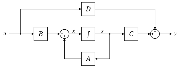
The state-space model (SSM) is defined by this simple equation. In general, SSM is modeled with a linear system that maps a 1-dimensional input signal $u (t)$ to an $N$-dimensional latent state $x(t)$ before projecting to a 1-dimensional output signal $y(t)$:
\[\begin{aligned} \dot{x}(t) & = \mathbf{A}(t) x(t) + \mathbf{B}(t) u(t) \\ y(t) & = \mathbf{C}(t) x(t) + \mathbf{D}(t) u(t) \end{aligned}\]where $\mathbf{A}(t) \in \mathbb{R}^{N \times N}$, $\mathbf{B}(t) = \mathbb{R}^{N \times 1}$, $\mathbf{C}(t) = \mathbb{R}^{1 \times N}$, $\mathbf{D} (t) \in \mathbb{R}$. In this general formulation, all matrices are allowed to be time-variant (i.e. their elements can depend on time); however, in the common LTI case, matrices will be time invariant, i.e. $\mathbf{A}(t) = \mathbf{A}$, $\mathbf{B}(t) = \mathbf{B}$, $\mathbf{C}(t) = \mathbf{C}$, and $\mathbf{D}(t) = \mathbf{D}$.
Discretization of SSM
Usually, we are interested in a discrete input sequence \(\{ u_{t_k} \}_{k \in \mathbb{N}}\) instead of continuous signal $u(t)$. In such scenarios, the SSM must be discretized by a step size $\Delta t$ that represents the resolution of the input. Many discretization methods for numerical integration of ODEs exist, and numerical integration methods are popular and the simplest methods.
Consider the standard setting of a first-order ODE for a continuous function $f (t, x)$:
\[\dot{x} (t) = f(t, x (t)) \text{ where } x(t_0) = x_0\]Numerical integration methods start from the equation:
\[x_k - x_{k-1} := x (t_k) - x (t_{k - 1}) = \int_{t_{k-1}}^{t_k} f (s, x (s)) \mathrm{d} s\]- Euler method
By the rectangle rule with left endpoint $t_{k-1}$, i.e. $f(s, x(s)) \approx f(t_{k-1}, x(t_{k-1}))$: $$ x_k - x_{k-1} = \Delta t_k \cdot f(t_{k-1}, x(t_{k-1})) \text{ where } \Delta t_k = t_k - t_{k-1} $$ - Backward Euler method
By the rectangle rule with right endpoint $t_k$, i.e. $f(s, x(s)) \approx f(t_k, x(t_k))$: $$ x_k - x_{k-1} = \Delta t_k \cdot f(t_k, x(t_k)) \text{ where } \Delta t_k = t_k - t_{k-1} $$ - Trapezoidal Rule
By the trapezoidal rule with midpoint $\frac{t_k + t_{k-1}}{2}$, i.e. $f(s, x(s)) \approx \frac{f(t_k, x(t_k)) + f(t_{k-1}, x(t_{k-1}))}{2}$: $$ x_k - x_{k-1} = \Delta t_k \cdot \frac{f(t_k, x(t_k)) + f(t_{k-1}, x(t_{k-1}))}{2} \text{ where } \Delta t_k = t_k - t_{k-1} $$ - Generalized Bilinear Transform (GBT)
By generalizing above rules with a convex combination of the left and right endpoints, weighing them by $1 − \alpha$ and $\alpha$ respectively: $$ x_k - x_{k-1} = \Delta t_k \cdot \left[ \alpha \cdot f(t_k, x(t_k)) + (1 - \alpha) \cdot f(t_{k-1}, x(t_{k-1}))\right] \text{ where } \Delta t_k = t_k - t_{k-1} $$
Applying GBT to our linear SSM $f(t, x(t)) = \mathbf{A} x(t) + \mathbf{B} u(t)$:
\[\begin{aligned} x_k - x_{k-1} & = \int_{t_{k-1}}^{t_k} \mathbf{A} x(s) \mathrm{d} s + \int_{t_{k-1}}^{t_k} \mathbf{B} u (s) \mathrm{d} s \\ & = \int_{t_{k-1}}^{t_k} \mathbf{A} x(s) \mathrm{d} s + \Delta t_k \mathbf{B} u_k \\ & \approx \Delta t_k \left[ (1- \alpha) \mathbf{A} x_{k-1} + \alpha \mathbf{A} x_k \right] + \Delta t_k \mathbf{B} u_k \end{aligned}\]where $u_k = \frac{1}{\Delta t_k} \int_{t_{k-1}}^{t_k}$ denotes the average value in each discrete time interval. Rearraging terms:
\[x_k = \underbrace{(\mathbf{I} - \alpha \Delta t_k \cdot \mathbf{A})^{-1} (\mathbf{I} + (1 - \alpha) \Delta t_k \cdot \mathbf{A})}_{\bar{\mathbf{A}}} x_{k-1} + \underbrace{(\mathbf{I} - \alpha \Delta t_k \cdot \mathbf{A})^{-1} \Delta t_k \cdot \mathbf{B}}_{\bar{\mathbf{B}}} u_k\]therefore \(y_k = \mathbf{C} x_k + \mathbf{D} u_k\).
Linear SSM as Deep Learning Layers
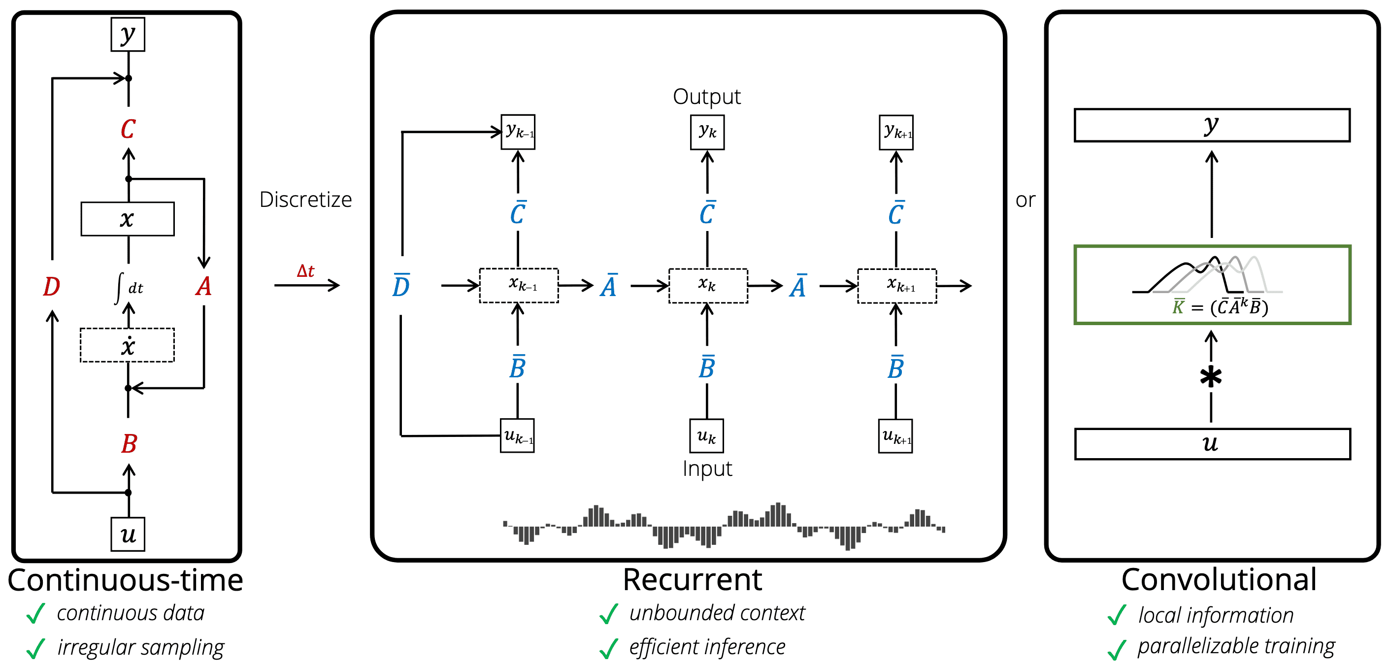
Gu et al. NeurIPS 2021 theoretically shows that deep learning layers (RNNs and CNNs) are closely related to the linear state-space models. Computationally, the discrete-time LSSL can be viewed in multiple ways as illustrated in the following figure:
Discrete-time SSM as RNNs
Considering $x_k$ in a discrete-time SSM as a hidden state with the transition matrix $\bar{\mathbf{A}}$, the linear SSM can be interpreted as a single-layer RNN. And the matrices $\bar{\mathbf{A}}$ and $\bar{\mathbf{B}}$ in the discrete-time LSSL function analogously to the gates $\sigma$, $1 - \sigma$. Furthermore, the following theorem shows that LSSLs and popular families of RNN methods are closely related in the sense that they all approximate the same continuous-time dynamics:
\[\dot{x}(t) = - x(t) + f(t, x(t))\]Consider the 1D gated RNN (e.g. LSTM, GRU): $$ x_k = (1 - \sigma (z_k)) x_{k-1} + \sigma (z_k) \bar{f} (k, x_{k-1}) $$ where $\sigma$ is the sigmoid function and $\bar{f}(k, x)$ is an arbitrary function that is Lipschitz in its second argument $x$. For example, a basic RNN could define $\bar{f}(k, x) = \tanh (\mathbf{W} x + \mathbf{U} u_k)$ (e.g., candidate hidden state of GRU), or simply $\bar{f} (k, x_{k-1}) = u_k$ as vanilla RNN. Then, it is a backwards Euler discretization with step sizes $\Delta t_k = \exp (z_k)$ of the following non-linear ODE: $$ \dot{x}(t) = - x(t) + f(t, x(t)) $$ Note that the linear SSM ($\bar{f} (k, x_{k-1}) = u_k$) also approximates this dynamics, and discretization with $\mathbf{A} = −1$, $\mathbf{B} = 1$, $\alpha = 1$ exactly produces the gated recurrence.
$\mathbf{Proof.}$
Applying the backwards Euler discretization:
\[x_k - x_{k - 1} = - \Delta t_k \cdot x_k + \Delta t_k \cdot f(t_k, x_k)\]which is equivalent to:
\[x_k = \frac{1}{1 + \Delta t_k} x_{k-1} + \frac{\Delta t_k}{1 + \Delta t_k} f(t_k, x_k)\]Note that $\frac{\Delta t_k}{1 + \Delta t_k} = \frac{1}{1 + \exp(-z_k)}$
\[\tag*{$\blacksquare$}\]Discrete-time Linear SSM as CNNs
The LSSL can be interpreted as automatically learning convolution filters with a flexible kernel width. Let $u \in \mathbb{R}^{L \times H}$ be an input vector with a sequence length $L$ where each timestep has an $H$-dimensional feature vector. For simplicity let the initial state be $x_{-1} = 0$. Then unrolling explicitly yields:
\[\begin{array}{llll} x_0 = \bar{\mathbf{B}} u_0 & x_1 = \bar{\mathbf{A} \mathbf{B}} u_0 + \bar{\mathbf{B}} u_1 & x_2 = \bar{\mathbf{A}}^2 \bar{\mathbf{B}} u_0 + \bar{\mathbf{A}} \bar{\mathbf{B}} u_1+ \bar{\mathbf{B}} u_2 & \ldots \\ y_0 = \mathbf{C} \bar{\mathbf{B}} u_0 + \mathbf{D} u_0 & y_1 = \mathbf{C} \bar{\mathbf{A}} \bar{\mathbf{B}} u_0 + \mathbf{C} \bar{\mathbf{B}} u_1 + \mathbf{D} u_1 & y_2 = \mathbf{C} \bar{\mathbf{A}}^2 \bar{\mathbf{B}} u_0 + \mathbf{C} \bar{\mathbf{A}} \bar{\mathbf{B}} u_1 + \mathbf{C} \bar{\mathbf{B}} u_2 + \mathbf{D} u_2 & \ldots \end{array}\]which implies:
\[y_k = \sum_{n=0}^{k} \mathbf{C} \bar{\mathbf{A}}^{k - n} \bar{\mathbf{B}} u_n + \mathbf{D} u_k\]Then the output $y$ is simply the (non-circular) convolution $y = \bar{\mathbf{K}} \ast u + \mathbf{D} u$ where the SSM convolution kernel (filter) $\bar{\mathbf{K}}$ is defined as:
\[\bar{\mathbf{K}} = \left(\mathbf{C} \bar{\mathbf{A}}^n \bar{\mathbf{B}}\right)_{n=0}^{L - 1} = (\mathbf{C} \bar{\mathbf{B}}, \mathbf{C} \bar{\mathbf{A}} \bar{\mathbf{B}}, \cdots, \mathbf{C} \bar{\mathbf{A}}^{L - 1} \bar{\mathbf{B}}) \in \mathbb{R}^L\]The result of applying this kernel can be computed either through a direct convolution or by leveraging convolution theorem with Fast Fourier Transform (FFT). The discrete convolution theorem, which pertains to the circular convolution of two sequences (for non-circular convolution, vectors $u$ and $\bar{\mathbf{K}}$ should be zero padded), enables an efficient calculation of the convolution output by first multiplying the FFTs of the input vectors, followed by applying an inverse FFT.
HiPPO: Recurrent Memory with Optimal Polynomial Projections
Previous work found that the basic SSM actually performs poorly in practice. One intuitive explanation is that linear first-order ODEs resolve into exponential functions, which may result in gradients scaling exponentially with sequence length (the vanishing or exploding gradients problem). A fundamental aspect of modeling long-term and complex temporal dependencies in modern machine learning is memory–storing and integrating information from previous timesteps. The main challenge with this approach is limited capacity to store the entire cumulative history. Furthermore, existing methods typically rely on prior knowledge of sequence length and fail to perform effectively outside of this length.
To address this memory problem, the LSSL leveraged the HiPPO theory of continuous-time memorization, which spectifies the class of transition matrix $\mathbf{A}$:
\[\texttt{HiPPO Matrix: } \mathbf{A}_{nk} = - \begin{cases} (2n + 1)^{\frac{1}{2}} (2k + 1)^{\frac{1}{2}} & \text{ if } n > k \\ n + 1 & \text{ if } n = k \\ n < k & \text{ if } n < k \end{cases}\]For example, the LSSL could be improved its performance on the sequential MNIST benchmark from $60\%$ to $98\%$ by simply modifying an SSM from a random matrix $\mathbf{A}$ to this equation.
The key insight of HiPPO proposed by Gu et al. NeurIPS 2020 is to reformulate the memorization as an online function approximation problem, where the input function $f (t): \mathbb{R}^+ \to \mathbb{R}$ at timestep $t$ is summarized by storing its optimal coefficients for the approximation with given basis functions.
Preliminary: Approximation Theory and Orthogonal Polynomials
Let \(f^*\) be an unknown target function that we’re interested in and usually intractable. In approximation theory, our goal is to construct an approximation of \(f^*\) by using tractable function $f$. Since polynomials are among the simplest functions, and because computers can directly evaluate polynomials, this is typically done by leveraging the polynomials $f_n (x) = \sum_{i=1}^n c_i x^i$ that reside on the function space \(\mathbb{P}_n = \textrm{span} \{ 1, x, x^2, \cdots x^n \}\). And the expressive power of polynomials are shown to be effective by various theorems, especially Weierstrass approximation theorem:
Let $f^* \in C([a, b], \mathbb{R})$ (continuous real-valued function). For any $\varepsilon > 0$, there exists $n \in \mathbb{N}$ and $p_n \in \mathbb{P}_n$ such that $\lVert f^* - p_n \rVert = \underset{x \in [a, b]}{\sup} \lvert f^* (x) - p_n (x) \rvert < \varepsilon$.
$\mathbf{Proof.}$
Without loss of generality, let $a=0$ and $b=1$. Since \(f^*\) is continuous on the compact set $[0,1]$, $f^*$ is bounded, hence we can set \(M = \lVert f^* \rVert < \infty\). Consequently, for any $\xi \in [0,1]$, the following holds:
\[\lvert f(x) - f(\xi) \rvert \leq \begin{cases} \cfrac{\varepsilon}{2} & & \text{ if } \lvert x - \xi \rvert < \delta \\ \lvert f(x) \rvert + \lvert f(\xi) \rvert & \leq 2M & \\ & \leq 2M \cdot 1 & \\ & \leq 2M \cdot \cfrac{\lvert x - \xi \rvert^2}{\delta^2} & \text{ otherwise } \end{cases}\]Hence we obtain
\[\lvert f(x) - f(\xi) \rvert \leq 2M \cdot \frac{\lvert x - \xi \rvert^2}{\delta^2} + \frac{\varepsilon}{2}\]Now, we will prove that the polynomial of interest is actually the Bernstein polynomial. Before the proof, the definition of Bernstein polynomial is given.
The $n+1$ Bernstein basis polynomials of degree $n$ are defined as $$ b_{\nu,n}(x)=\binom{n}{\nu} x^\nu (1−x)^{n−\nu} \text{ where } \nu = 0,\cdots, n. $$ The first few Bernstein basis polynomials from above in monomial form are: $$ \begin{array}{lll} b_{0,0}(x)=1, & & \\ b_{0,1}(x)=1-1 x, & b_{1,1}(x)=0+1 x & & \\ b_{0,2}(x)=1-2 x+1 x^2, & b_{1,2}(x)=0+2 x-2 x^2, & b_{2,2}(x)=0+0 x+1 x^2 & \end{array} $$ A Bernstein polynomial is a linear combination of Bernstein basis polynomials: $$ B_n(x) = \sum_{\nu = 0}^n \beta_\nu b_{\nu,n}(x) $$ where the coefficients $\beta_\nu$ are called Bernstein coefficients. In the proof, we will use the following Bernstein polynomial induced by continuous function $f: [0, 1] \to \mathbb{R}$: $$ B_n (x ; f) \sum_{\nu = 0}^n f \left( \frac{\nu}{n} \right) b_{\nu,n}(x) $$
Note that the last line is due to the properties of Bernstein polynomials: $B_n (x; x^2) = x^2 + \cfrac{1}{n} (x - x^2)$ and $B_n(x;af+g)=aB_n(x;f)+B_n(x;g)$. Next, let $\xi=x$. Then consequently,
\[\begin{aligned} \left|B_n(x ; f)-f(x)\right| & \leq \frac{2 M}{\delta^2} \cdot \frac{\xi - \xi^2}{n} + \frac{\varepsilon}{2} \\ & \leq \frac{M}{2 \delta^2} \cdot \frac{1}{n} + \frac{\varepsilon}{2} \end{aligned}\]By choosing large $n$ such that $n \geq \frac{M}{\delta^2 \varepsilon}$, for any $x \in [0, 1]$, we have
\[\begin{aligned} \left|B_n(x ; f)-f(x)\right| & \leq \varepsilon \end{aligned}\]and equivalently
\[\begin{aligned} \lVert B_n(\cdot ; f) - f\rVert & \leq \varepsilon. \end{aligned}\] \[\tag*{$\blacksquare$}\]For polynomial basis, orthogonal polynomials (OPs) are widely used since they offer several advantages in constructing accurate and efficient approximations of functions. It is a family of polynomials such that any two different polynomials in the sequence are orthogonal to each other under some inner product.
Given any measure $\mu$, a sequence of polynomials $\{ p_n (x) : \mathbb{R} \to \mathbb{R} \vert n = 0, 1, \cdots \}$ is orthogonal polynomials if the following are satisfied:
- $\textrm{deg } p_n = n$;
- $\left< p_n, p_m \right> = \int p_n p_m \; d\mu = 0 \quad \text{ for } \quad n \neq m$;
- $\left< p_n, p_n \right> = 1$.
For example, we can use orthogonal bases to construct good approximations for unknown target function $f$. Suppose that \(\{p_j \}\) is a polynomial basis, but not necessarily orthogonal, and we want to find the approximation coefficients $\mathbf{c}$:
\[f \approx \sum_{j=1}^N c_j p_j \text{ minimizes } \left\Vert f - \sum_{j=1}^N c_j p_j \right\Vert_{w}\]To find the coefficients, consider the critical point:
\[0 = \frac{\partial}{\partial c_i} \int \left( f - \sum_{j=1}^N c_j p_j \right)^2 w (x) \mathrm{d}x = - 2 \int \left( f - \sum_{j=1}^N c_j p_j \right) p_i w (x) \mathrm{d} x\]which is equivalent to:
\[\begin{gathered} \int f(x) p_i (x) w(x) \mathrm{d} x = \sum_{j=1}^n \left( \int p_i p_j w (x) \mathrm{d}x \right) c_j \\ \Big\Downarrow \\ \langle f, p_i \rangle_w = \langle p_i, p_j \rangle_w c_j \\ \end{gathered}\]In matrix form, this relation is a linear system $\mathbf{A} \mathbf{c} = \mathbf{f}$ where \(\mathbf{a}_{ij} = \langle p_i, p_j \rangle_w\) and \(\mathbf{f}_{i} = \langle f, p_i \rangle_w\). If the basis is orthogonal, then the matrix reduces to a diagonal system and the solution is just:
\[c_i = \frac{\langle f, p_i \rangle_w}{\langle p_i, p_i \rangle_w}\]Therefore, exploiting the structure of the orthogonal basis can be a good starting point for building numerical approximations.
HiPPO framework
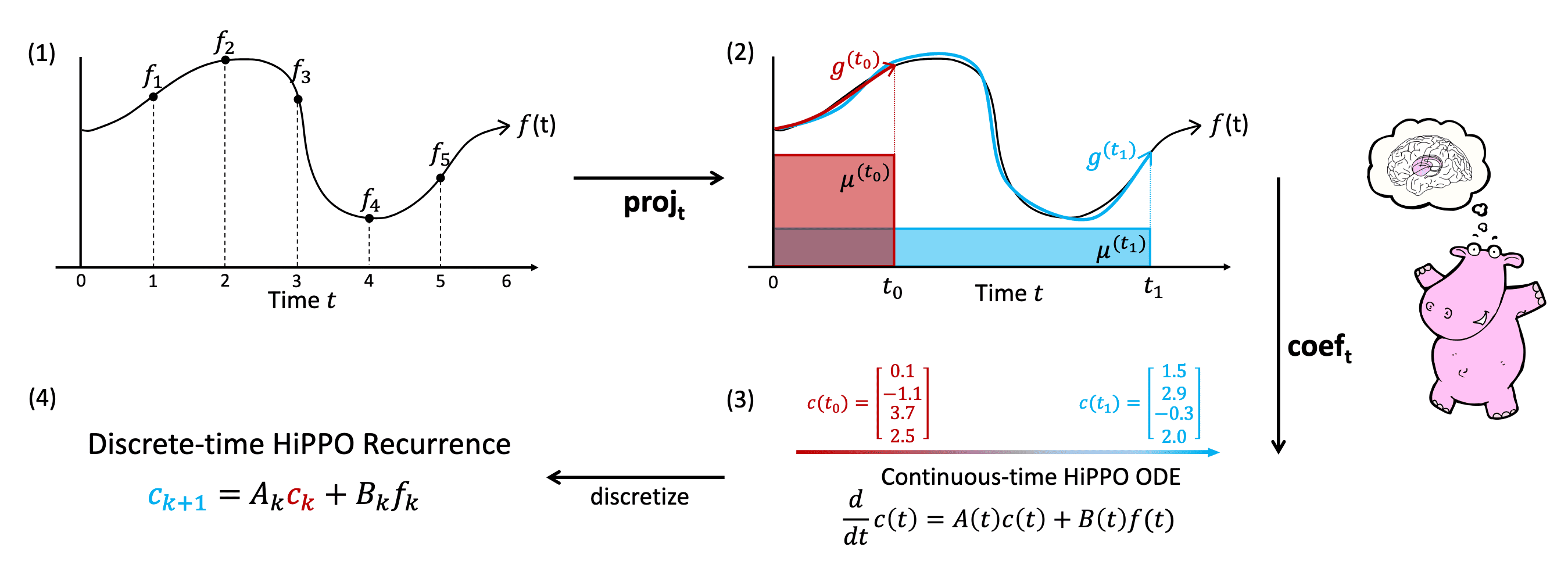
Given an input function $f(t) \in \mathbb{R}$ on continuous timesteps $t \geq 0$, we are interested in operating on the cumulative history \(f_{\leq t} := f(x) \vert_{x \leq t}\). Since the space of functions is intractably large, the history cannot be perfectly memorized and must be compressed.
Since we care about approximating $f_{\leq t}$ for every time $t$, HiPPO (High-order Polynomial Projection Operators) aims to find the well-compressed history $g^{(t)}$ by projecting $f_{\leq t}$ onto the subspace $\mathcal{G}$ of orthogonal polynomials \(\{ g_n \}_{n=1}^N\), which minimizes:
\[\Vert f_{\leq t} - g^{(t)} \Vert_{L_2 (\mu^{(t)})} := \sqrt{\int_0^\infty f_{\leq t} g^{(t)} \mathrm{d} \mu^{(t)} }\]for each time $t$ where $\mu^{(t)}$ is a measure supported on $(-\infty, t]$. For this online function approximation, the HiPPO framework can be formally defined with the following two operators:
Given any time-varying measure family $\mu^{(t)}$ supported on $(−\infty,t]$, HiPPO defines a projection operator $\texttt{proj}_t$ and a coefficient extraction operator $\texttt{coef}_t$ at every time $t$:
- $\texttt{proj}_t$ takes function $f$ restricted up to time $t$, $f_{\leq_t} := f(x) \vert_{x \leq t}$, and maps it to a polynomial $g^{(t)} \in \mathcal{G}$, that minimizes the approximation error: $$ \Vert f_{\leq t} - g^{(t)} \Vert_{L_2 (\mu^{(t)})} := \sqrt{\int_0^\infty f_{\leq t} g^{(t)} \mathrm{d} \mu^{(t)} } $$
- $\texttt{coef}_t: \mathcal{G} \to \mathbb{R}^N$ maps the polynomial $g^{(t)}$ to the coefficients $c(t) \in \mathbb{R}^N$ of the basis of orthogonal polynomials defined with respect to the measure $\mu^{(t)}$: $$ g^{(t)} := \underset{g \in \mathcal{G}}{\arg \min} \Vert f_{\leq t} - g^{(t)} \Vert_{\mu^{(t)}} = \sum_{n=0}^{N - 1} c_n (t) g_n^{(t)} $$
With specific instantiations we will see in the next section, HiPPO maintains the linear ODE for the coefficient function $c(t)$:
\[\frac{\mathrm{d}}{\mathrm{d} t} c (t) = A(t) c(t) + B(t) f(t)\]By discretizing the coefficient dynamics, HiPPO yields an efficient closed-form recurrence \(\{ c_k \}_{k \in \mathbb{N}}\) for online compression of time series $( f_k )_{k\in \mathbb{N}}$.
HiPPO Instantiations
The main theoretical results of HiPPO are instantiations for various measure families $\mu^{(t)}$.

Translated Legendre (LegT) & Translated Laguerre (LagT)
Inspired from the sliding window, the translated Legendre (LegT) measures assign uniform weight to the most recent history $[t− \theta,t]$ and the translated Laguerre (LagT) measures assign exponentially decaying weight, which prioritizes recent history:
\[\begin{aligned} \texttt{LegT: } \mu^{(t)} (x) & = \frac{1}{\theta} \mathbb{I}_{[t - \theta, t]} (x) \\ \texttt{LagT: } \mu^{(t)} (x) & = e^{-(t-x)} \mathbb{I}_{(- \infty, t]} (x) = \begin{cases} e^{x - t} & \text{ if } x \leq t \\ 0 & \text{ if } x > t \end{cases} \\ \end{aligned}\]Then, with the Legendre and Laguerre polynomials, the linear cofficient dynamics are guaranteed:
- HiPPO-LegT
For LegT measures, define the orthogonal polynomial basis with Legendre polynomials $P_n (x)$ as follows: $$ g_n (t, x) = \lambda_n p_n (t, x) \text{ where } \begin{aligned}[t] p_n (t, x) & = (2n+1)^{\frac{1}{2}} P_n \left( \frac{2 (x-t)}{\theta} + 1 \right) \\ \lambda_n & = (2n + 1)^{\frac{1}{2}} (-1)^{n} \end{aligned} $$ where $p_n^{(t)}$ is the normalized version of $P_n^{(t)}$. Then, the $\texttt{hippo}$ operators are given by LTI ODEs: $$ \frac{\mathrm{d}}{\mathrm{d} t} c(t) = - A c(t) + B f(t) $$ where $A \in \mathbb{R}^{N \times N}$ and $B \in \mathbb{R}^{N}$: $$ A_{n k}=\frac{1}{\theta}\left\{\begin{array}{ll} (-1)^{n-k}(2 n+1) & \text { if } n \geq k \\ 2 n+1 & \text { if } n \leq k \end{array}, \quad B_n=\frac{1}{\theta}(2 n+1)(-1)^n\right. $$ - HiPPO-LagT
For LagT measures, define the orthogonal polynomial basis with Laguerre polynomials $L_n^{(\alpha)}$ as follows: $$ g_n (t, x) = \lambda_n p_n (t, x) \text{ where } \begin{aligned}[t] p_n (t, x) & = \frac{\Gamma (n + 1)^{\frac{1}{2}}}{\Gamma (n+ \alpha + 1)^{\frac{1}{2}}} L_n^{(\alpha)} (t - x) \\ \lambda_n & = \frac{\Gamma (n + \alpha + 1)^{\frac{1}{2}}}{\Gamma (n+1)^{\frac{1}{2}}} \end{aligned} $$ where $p_n^{(t)}$ is the normalized version of $L_n^{(\alpha)} (t - x)$. Then, the $\texttt{hippo}$ operators are given by LTI ODEs: $$ \frac{\mathrm{d}}{\mathrm{d} t} c(t) = - A c(t) + B f(t) $$ where $A \in \mathbb{R}^{N \times N}$ and $B \in \mathbb{R}^{N}$: $$ A_{n k}=\left\{\begin{array}{ll} 1 & \text { if } n \geq k \\ 0 & \text { if } n < k \end{array}, \quad B_n=1\right. $$
$\mathbf{Proof.}$
For brevity, we prove LegT case only since the statement for LagT measures can be proved in analogous way. Please refer to the appendix of the original paper for the proof of LagT measures.
LegT
Note that the derivative of the LegT measure is:
\[\frac{\partial \mu^{(t)} (x)}{\partial t} = \frac{1}{\theta} \delta_t - \frac{1}{\theta} \delta_{t- \theta}\] \[\begin{aligned} \frac{\partial g_n (t, x)}{\partial t} & = \lambda_n (2n + 1)^\frac{1}{2} \cdot \frac{-2}{\theta} P_n^\prime \left( \frac{2 (x - t)}{\theta} + 1 \right) \\ & = \lambda_n (2n + 1)^\frac{1}{2} \cdot \frac{-2}{\theta} \left[ (2n - 1) P_{n-1}^\prime \left( \frac{2 (x - t)}{\theta} + 1 \right) + (2n - 5) P_{n-3}^\prime \left( \frac{2 (x - t)}{\theta} + 1 \right) + \cdots \right] \\ & = - \lambda_n (2n + 1)^\frac{1}{2} \cdot \frac{2}{\theta} \left[ \lambda_{n-1}^{-1} (2n - 1)^{\frac{1}{2}} g_{n-1} (t, x) + \lambda_{n-3}^{-1} (2n - 3)^{\frac{1}{2}} g_{n-3} (t, x) + \cdots \right] \\ \end{aligned}\]From the preliminary, recall that the optimal approximation coefficients of orthogonal polynomials are given by $c_n (t) = \langle f_{\leq t}, g_n^{(t)} \rangle / \langle g_n^{(t)}, g_n^{(t)} \rangle$. Without loss of generality, the authors defined the optimal coefficient as $c_n (t) = \langle f_{\leq t}, g_n^{(t)} \rangle_{\mu^{(t)}}$ by incorporating the normalization factor into the function:
\[f_{\leq t} \approx \sum_{n=0}^{N - 1} \underbrace{\langle f_{\leq t}, g_n^{(t)} \rangle_{\mu^{(t)}}}_{c_n (t)} \frac{g_{n}^{(t)}}{\Vert g_n^{(t)} \Vert_{\mu^{(t)}}^2}\]Therefore:
\[c_n (t) = \lambda_n \int f p_n^{(t)} \mathrm{d} \mu^{(t)} = \int f g_n^{(t)} \mathrm{d} \mu^{(t)}\]Using Leibniz Integral rule, we have:
\[\begin{aligned} \frac{\mathrm{d}}{\mathrm{d} t} c_n (t) & = \begin{aligned}[t] & \int f (x) \left( \frac{\partial g_n (t, x)}{\partial t} \right) \mathrm{d} \mu^{(t)} (x) \\ & + \int f (x) g_n (t, x) \left( \frac{\partial x \mu^{(t)} (x)}{\partial t} \right) \mathrm{d} x \end{aligned} \\ & = \begin{aligned}[t] & \frac{1}{\theta} f(t) g_n (t, t) - \frac{1}{\theta} f(t-\theta) g_n(t, t-\theta) \\ & - \lambda_n (2n + 1)^{\frac{1}{2}} \frac{2}{\theta} \left[\lambda_{n-1}^{-1} (2 n - 1)^{\frac{1}{2}} c_{n - 1} (t) + \lambda_{n-3}^{-1} (2n-5)^{\frac{1}{2}} c_{n-3} (t) + \cdots \right] \end{aligned} \\ \end{aligned}\]Note that:
\[\begin{aligned} g_n (t, t) & = \lambda_n (2n + 1)^\frac{1}{2} \\ g_n (t, t-\theta) & = \lambda_n (-1)^n (2n + 1)^\frac{1}{2} \end{aligned}\]Additionally, observe that the value $f(t - \theta)$ is required, which is no longer available at time $t$. Instead, we approximate using $f_{\leq t}$:
\[\begin{aligned} f_{\leq t} (x) & \approx \sum_{k=0}^{N-1} \lambda_k^{-1} c_k (t) (2k+1)^{\frac{1}{2}} P_k \left( \frac{2 (x - t)}{\theta} + 1 \right)\\ \Rightarrow f(t-\theta) & \approx \sum_{k=0}^{N-1} \lambda_k^{-1} c_k (t) (2k+1)^{\frac{1}{2}} (-1)^k \end{aligned}\]Then:
\[\begin{aligned} \frac{\mathrm{d}}{\mathrm{d} t} c_n (t) & \approx \begin{aligned}[t] & (2n + 1)^{\frac{1}{2}} \frac{\lambda_n}{\theta} f(t) - (2n + 1)^{\frac{1}{2}} \frac{\lambda_n}{\theta} (-1)^n \sum_{k=0}^{N - 1} (2k + 1)^{\frac{1}{2}} \frac{c_k (t)}{\lambda_k} (-1)^k \\ & - \lambda_n (2n + 1)^{\frac{1}{2}} 2 \left[\lambda_{n-1}^{-1} (2 n - 1)^{\frac{1}{2}} \frac{c_{n - 1} (t)}{\lambda_{n-1}} + (2n-5)^{\frac{1}{2}} \frac{c_{n-3} (t)}{\lambda_{n-3}} + \cdots \right] \end{aligned} \\ & = - \frac{\lambda_n}{\theta} (2n + 1)^{\frac{1}{2}} \sum_{k=0}^{N-1} M_{nk} (2k + 1)^{\frac{1}{2}} \frac{c_k (t)}{\lambda_k} + (2n + 1)^{\frac{1}{2}} f(t) \end{aligned}\]where
\[M_{nk} = \begin{cases} 1 & \text{ if } k \leq n \\ (-1)^{n-k} & \text{ if } k \geq n \end{cases}\]By plugging in $\lambda_n$ into the equation, done.
\[\tag*{$\blacksquare$}\]Scaled Legendre (LegS)
To avoid forgetting, the memory should scale the window over time. For this intuition, the scaled Legendre (LegS) measure assigns uniform weight to all history $[0, t]$:
\[\mu^{(t)} = \frac{1}{t} \mathbb{I}_{[0, t]}\]For LegS measures, define the orthogonal polynomial basis with Legendre polynomials $P_n (x)$ as follows: $$ g_n (t, x) = p_n (t, x) \text{ where } \begin{aligned}[t] p_n (t, x) & = (2n+1)^{\frac{1}{2}} P_n \left( \frac{2 (x-t)}{\theta} + 1 \right) \\ \end{aligned} $$ where $p_n^{(t)}$ is the normalized version of $P_n^{(t)}$. Then, the $\texttt{hippo}$ operators are given by LTI ODEs: $$ \frac{\mathrm{d}}{\mathrm{d} t} c(t) = - \frac{1}{t} A c(t) + \frac{1}{t} B f(t) $$ where $A \in \mathbb{R}^{N \times N}$ and $B \in \mathbb{R}^{N}$: $$ A_{n k}=\left\{\begin{array}{ll} (2n+1)^{\frac{1}{2}} (2k+1)^{\frac{1}{2}} & \text { if } n > k \\ n+1 & \text { if } n = k \\ 0 & \text{ if } n < k \end{array}, \quad B_n=(2 n+1)^{\frac{1}{2}} \right. $$
$\mathbf{Proof.}$
Note that:
\[g_n (t, t) = (2n + 1)^{\frac{1}{2}} P_n (1) = (2n + 1)^{\frac{1}{2}}\]Again, differentiate the measure and basis:
\[\begin{aligned} \frac{\partial \mu^{(t)} (x)}{\partial t} & = - t^{-2} \mathbb{I}_{[0, t]} + t^{-1} \delta_t \\ \frac{\partial g_n (t, x)}{\partial t} & = - (2n + 1)^{\frac{1}{2}} 2x t^{-2} P_n^\prime \left(\frac{2x}{t} - 1 \right) \\ & = - (2n + 1)^{\frac{1}{2}} t^{-1} \left( \frac{2x}{t} - 1 + 1 \right) P_n^\prime \left(\frac{2x}{t} - 1 \right) \end{aligned}\]Denote $z = \frac{2x}{t} - 1$ and apply the properties of derivatives of Legendre polynomials:
\[\begin{aligned} \frac{\partial g_n (t, x)}{\partial t} & - (2n + 1)^{\frac{1}{2}} t^{-1} (z + 1) P_n^\prime (z) \\ & = - (2n + 1)^{\frac{1}{2}} t^{-1} \left[ n P_n (z) + (2n-1) P_{n-1}(z) + (2n-3) P_{n-2}(z) + \cdots \right] \\ & = - (2n + 1)^{\frac{1}{2}} t^{-1} \left[ n (2n + 1)^{-\frac{1}{2}} g_n (t, x) + (2n-1)^{\frac{1}{2}} g_{n-1}(t, x) + (2n-3)^{\frac{1}{2}} g_{n-2}(t, x) + \cdots \right] \\ \end{aligned}\]By differentiating \(c_n (t) = \langle f, g_n^{(t)} \rangle_{\mu^{(t)}}\) with Leibniz rule and plugging the derivatives into the equation, the theorem will be derived.
\[\tag*{$\blacksquare$}\]S4: Structured State Space for Sequence Modeling
The LSSL conceptually integrates the strengths of Continuous-Time Model (CTM), RNN and CNN, and offers a proof of concept that deep SSMs with HiPPO theory can, in principle, address long range dependencies. However, the LSSL is infeasible to use in practice since realizing these conceptual advantages requires the use of different parameter representations that are computationally far more expensive compared to RNNs and CNNs.

Gu et al. ICLR 2022 introduced the Structured State Space sequence (S4) model built upon the SSM that overcomes the critical computational bottleneck. Its novel parameterization that efficiently swaps among continuous-time state space/recurrence/convolution representations enables it to handle a wide range of tasks, be efficient at both training and inference, and excel in processing long sequences.
Preliminary: Diagonalization of LSSM
The fundamental bottleneck in computing the discrete-time SSM is that it involves repeated matrix multiplication by $\bar{\mathbf{A}}$. For example, computing SSM convolution kernel $\bar{\mathbf{K}} = \left(\mathbf{C} \bar{\mathbf{A}}^n \bar{\mathbf{B}}\right)_{n=0}^{L - 1}$ naively as in the LSSL involves $L$ successive multiplications by $\bar{\mathbf{A}}$, requiring $\mathcal{O}(N^2 L)$ operations and $\mathcal{O}(N L)$ space.
The S4 parameterization starts from the motivation of diagonalization of $\mathbf{A}$. Consider a change of basis by $\mathbf{V}$ in the state $x = \mathbf{V} \tilde{x}$. Then, the two SSMs become identical:
\[\begin{array}{ll} x^\prime = \mathbf{A} x + \mathbf{B} u \quad & \tilde{x}^\prime = \mathbf{V}^{-1} \mathbf{A} \mathbf{V} \tilde{x} + \mathbf{V}^{-1} \mathbf{B} u \\ y = \mathbf{C} x \quad & y = \mathbf{C} \mathbf{V} \tilde{x} \end{array}\]Consequently, the conjugation is an equivalence relation on SSMs; $(\mathbf{A}, \mathbf{B}, \mathbf{C}) \sim (\mathbf{V}^{-1} \mathbf{A}, \mathbf{B}, \mathbf{C})$, which motivates putting $\mathbf{A}$ into a canonical form.
S4 Parameterization: Normal & Diagonal Plus Low-Rank (NPLR & DPLR)
However, in practice, the form of the SSM matrices $\mathbf{A}$ are impractical to diagonalize; for example, the authors showed that the diagonalization matrix $\mathbf{V}$ of HiPPO matrix imposes memory exponentially large in the state size $N$. This implies that we should only conjugate $\mathbf{A}$ by well-conditioned matrices $\mathbf{V}$, e.g. when $\mathbf{A}$ is normal (\(\mathbf{A}^* \mathbf{A} = \mathbf{A} \mathbf{A}^*\)) that is diagonalizable with unitary \(\mathbf{V} = \mathbf{V}^*\) by spectral theorem:
$\mathbf{A}$ is normal if and only if there exists a unitary matrix $\mathbf{V}$ such that $\mathbf{A} = \mathbf{V} \mathbf{\Lambda} \mathbf{V}^*$ where $\mathbf{\Lambda}$ is a diagonal matrix.
Instead of normal matrix, the authors showed that the SSM has special structure in $\mathbb{C}$ that can be decomposed as the sum of normal and low-rank factorization $\mathbf{P} \mathbf{Q}^\top$, which is termed Normal Plus Low-Rank (NPLR):
\[\mathbf{A} = \mathbf{V} \mathbf{\Lambda} \mathbf{V}^* - \mathbf{P} \mathbf{Q}^\top\]By equivalence relation, these NPLR matrices can be conjugated into diagonal plus low-rank (DPLR) form:
\[\mathbf{A} = \mathbf{\Lambda} - \mathbf{P} \mathbf{Q}^\top\]Under this special form, S4 overcomes the computational bottleneck of LSSL as follows:
S4 Convolution Layer
S4 overcomes the computational bottleneck of convolution by $\bar{\mathbf{K}}$ in three steps:
- SSM Generating Functions
Instead of computing $\bar{\mathbf{K}}$ directly: $$ \bar{\mathbf{K}} = \left( \mathbf{C}^* \bar{\mathbf{B}}, \mathbf{C}^* \bar{\mathbf{A}} \bar{\mathbf{B}}, \cdots, \mathbf{C}^* \bar{\mathbf{A}}^{L - 1} \bar{\mathbf{B}} \right) \in \mathbb{R}^L $$ the authors first introduce a generating function. The SSM generating function at node $z \in \mathbb{C}$ is defined as: $$ \begin{aligned} \hat{\mathbf{K}} (z ; \bar{\mathbf{A}}, \bar{\mathbf{B}}, \mathbf{C}) & := \sum_{n=0}^\infty \mathbf{C}^* \bar{\mathbf{A}}^n \bar{\mathbf{B}} z^n = \mathbf{C}^* \left( \mathbf{I} - \bar{\mathbf{A}} z \right)^{-1} \bar{\mathbf{B}} \\ \hat{\mathbf{K}}_L (z ; \bar{\mathbf{A}}, \bar{\mathbf{B}}, \mathbf{C}) & := \sum_{n=0}^L \mathbf{C}^* \bar{\mathbf{A}}^n \bar{\mathbf{B}} z^n = \mathbf{C}^* \left( \mathbf{I} - \bar{\mathbf{A}}^L z^L \right) \left( \mathbf{I} - \bar{\mathbf{A}} z \right)^{-1} \bar{\mathbf{B}} \end{aligned} $$ from the fact that $\mathbf{I} + \mathbf{A} + \mathbf{A}^2 + \cdots = (\mathbf{I} - \mathbf{A})^{-1}$. In vector form with $\Omega \in \mathbb{C}^M$: $$ \hat{\mathbf{K}} (\Omega ; \bar{\mathbf{A}}, \bar{\mathbf{B}}, \mathbf{C}) := \left( \hat{\mathbf{K}} (\Omega_k ; \bar{\mathbf{A}}, \bar{\mathbf{B}}, \mathbf{C}) \right)_{k=1}^M $$ Then, the SSM convolution filter $\bar{\mathbf{K}}$ can be recovered from evaluations of its generating function $\hat{\mathbf{K}}$ at the roots of unity $\Omega = \{ \exp ( 2\pi \frac{k}{L} ) \vert k = 1, \cdots, L \}$. Observe that the SSM generating function can be obtained through (Discrete) Fourier Transform: $$ \begin{aligned} \hat{\mathbf{K}} (\Omega_j) & = \sum_{n=0}^{L-1} \bar{\mathbf{K}}_n \underbrace{\exp \left( - 2\pi i \frac{nj}{L} \right)}_{\Omega_j^n} = \mathbf{C}^* \left( \mathbf{I} - \bar{\mathbf{A}}^L \Omega_j^L \right) \left( \mathbf{I} - \bar{\mathbf{A}} \Omega_j \right)^{-1} \bar{\mathbf{B}} \\ \Rightarrow \hat{\mathbf{K}} & = \mathcal{F}_L (\bar{\mathbf{K}}) \end{aligned} $$ from the fact that $$ (\mathbf{I} - \bar{\mathbf{A}} z) \sum_{n=0}^{L-1} \bar{\mathbf{A}}^k z^k = \mathbf{I} - \bar{\mathbf{A}}^L z^L $$ Therefore $\bar{\mathbf{K}}$ can be $\hat{\mathbf{K}}$ with a single inverse DFT, which requires $\mathcal{O}(L \log L)$ operations with the Fast Fourier Transform (FFT) algorithm. In summary, computing the SSM kernel is equivalent to computing the SSM generating function and this allows us to replace the matrix power with an single inverse. - Cauchy kernel
However, we still need to calculate the matrix inverse, which is known to require approximately $\mathcal{O} (n^{2.8})$. Hence, the next step is to assume special structure (DPLR) on $\mathbf{A}$ to compute the inverse faster. We first consider the diagonal case first. And let $\bar{\mathbf{A}}$ and $\bar{\mathbf{B}}$ be the SSM matrices $\mathbf{A}$ and $\mathbf{B}$ discretized by the bilinear discretization with step size $\Delta$. Recall that: $$ \begin{aligned} \bar{\mathbf{A}} & = \left( \mathbf{I} - \frac{\Delta}{2} \mathbf{A} \right)^{-1} \left( \mathbf{I} + \frac{\Delta}{2} \mathbf{A} \right) \\ \bar{\mathbf{B}} & = \left( \mathbf{I} - \frac{\Delta}{2} \mathbf{A} \right)^{-1} \Delta \cdot \mathbf{B} \end{aligned} $$ Then, by simple matrix multiplications, we can obtain: $$ \hat{\mathbf{K}}_\mathbf{A} (z) = \mathbf{C}^* \left( \mathbf{I} - \bar{\mathbf{A}} z \right)^{-1} \bar{\mathbf{B}} = \frac{2 \Delta}{1+z} \mathbf{C}^* \left[ 2 \frac{1-z}{1+z} \mathbf{I} - \Delta \cdot \mathbf{A} \right]^{-1} \mathbf{B} $$ If $\mathbf{A} = \mathbf{\Lambda}$ is diagonal, we can re-write the SSM generating function as the weighted dot product: $$ \begin{aligned} \hat{\mathbf{K}}_\mathbf{\Lambda} (z) = \underbrace{\frac{2 }{1+z}}_{a(z)} \sum_{i=1}^N \frac{\mathbf{C}_i \cdot \mathbf{B}_i}{\underbrace{\frac{2}{\Delta} \frac{1-z}{1+z}}_{b(z)} - \mathbf{\Lambda}_{ii}} \end{aligned} $$ This is exactly the same as Cauchy matrix $\mathbf{M}$, which is a well-studied problem with fast and stable numerical algorithms: $$ \mathbf{M} \in \mathbb{C}^{M \times N} = \frac{1}{\omega_i - \lambda_j} $$ Consequently, computing $\hat{\mathbf{K}}_\mathbf{\Lambda} (\omega_i)$ over all $\Omega$ is therefore exactly a Cauchy matrix-vector multiplication. - Woodbury Correction
Finally, we relax the diagonal assumption into DPLR $\mathbf{A} = \mathbf{\Lambda} - \mathbf{P}\mathbf{Q}^*$ with the low-rank component $\mathbf{P}, \mathbf{Q} \in \mathbb{C}^{N \times r}$. Using Woodbury Formula: $$ (\mathbf{\Lambda} + \mathbf{P} \mathbf{Q}^*)^{-1} = \mathbf{\Lambda}^{-1} - \mathbf{\Lambda}^{-1} \mathbf{P} (\mathbf{I}_r + \mathbf{Q}^* \mathbf{\Lambda}^{-1} \mathbf{P})^{-1} \mathbf{Q}^{-1} \mathbf{\Lambda}^{-1} $$ Consequently, we can correct the SSM generating function with additional 3 dot products: $$ \begin{aligned} \mathbf{C}^* \left( \mathbf{I} - \bar{\mathbf{A}} z \right)^{-1} \bar{\mathbf{B}} & = \frac{2}{1 + z} \mathbf{C}^* \left( \frac{2}{\Delta} \frac{1-z}{1+z} \mathbf{I} - \mathbf{A} \right)^{-1} \mathbf{B} \\ & = \frac{2}{1 + z} \mathbf{C}^* \left( \frac{2}{\Delta} \frac{1-z}{1+z} \mathbf{I} - \mathbf{\Lambda} + \mathbf{P} \mathbf{Q}^* \right)^{-1} \mathbf{B} \\ & = a(z) \left[ \frac{\mathbf{C}^* \mathbf{B}}{b(z)} - \frac{\mathbf{C}^* \mathbf{P}}{b(z)} \cdot \left(1 + \frac{\mathbf{Q}^* \mathbf{P}}{b(z)} \right)^{-1} \frac{\mathbf{Q}^* \mathbf{B}}{b(z)} \right] \end{aligned} $$ The following pseudocode summarizes these steps:
$\mathbf{Fig\ 7.}$ S4 Convolution Kernel (Sketch) (Gu et al. 2022)
S4 Recurrence Layer
We will leverage the fact that the inverse of a DPLR matrix is also DPLR (e.g. also by the Woodbury Formula). And assuming that the state matrix $\mathbf{A} = \mathbf{\Lambda} - \mathbf{P} \mathbf{Q}^*$ is DPLR overt $\mathbb{C}$, we can explicitly write out a closed form for the discretized matrix $\bar{\mathbf{A}}$ within reasonable complexity.
Recall that the discretized SSM matrices are given by:
\[\begin{aligned} \bar{\mathbf{A}} & = \left( \mathbf{I} - \frac{\Delta}{2} \mathbf{A} \right)^{-1} \left( \mathbf{I} + \frac{\Delta}{2} \mathbf{A} \right) \\ \bar{\mathbf{B}} & = \left( \mathbf{I} - \frac{\Delta}{2} \mathbf{A} \right)^{-1} \Delta \cdot \mathbf{B} \end{aligned}\]Forward Discretization
The second factor of $\bar{\mathbf{A}}$ is simplfied as:
\[\begin{aligned} \mathbf{I} + \frac{\Delta}{2} \mathbf{A} & = \mathbf{I} + \frac{\Delta}{2} \left( \mathbf{\Lambda} - \mathbf{P} \mathbf{Q}^* \right) \\ & = \frac{\Delta}{2} \left[ \frac{2}{\Delta} + \left( \mathbf{\Lambda} - \mathbf{P} \mathbf{Q}^* \right) \right]_{\mathbf{A}_0} \end{aligned}\]Second Discretization
The first inverse factor of $\bar{\mathbf{A}}$ is simplfied using Woodbury formula:
\[\begin{aligned} \left( \mathbf{I} - \frac{\Delta}{2} \mathbf{A} \right)^{-1} & = \left( \mathbf{I} - \frac{\Delta}{2} \left( \mathbf{\Lambda} - \mathbf{P} \mathbf{Q}^* \right) \right)^{-1} \\ & = \frac{2}{\Delta} \left[ \underbrace{\frac{2}{\Delta} - \mathbf{\Lambda}}_{\mathbf{U}} + \mathbf{P}\mathbf{Q}^* \right]^{-1} \\ & = \frac{2}{\Delta} \left[ \mathbf{U}^{-1} - \mathbf{U}^{-1} \mathbf{P} \left( \mathbf{I} + \mathbf{Q}^* \mathbf{U}^{-1} \mathbf{P} \right)^{-1} \mathbf{Q}^* \mathbf{U}^{-1} \right] \\ & \equiv \frac{2}{\Delta} \mathbf{A}_1 \end{aligned}\]Note that $\mathbf{A}_0$, $\mathbf{A}_1$ are accessed only through matrix-vector multiplications. Since they are both DPLR, they have $\mathcal{O}(N)$ matrix-vector multiplication. Therefore, the full bilinear discretization can be rewritten in terms of these matrices as:
\[\begin{aligned} \bar{\mathbf{A}} & = \mathbf{A}_1 \mathbf{A}_0 \\ \bar{\mathbf{B}} & = \frac{2}{\Delta} \mathbf{A}_1 \Delta \mathbf{B} = 2 \mathbf{A}_1 \mathbf{B} \end{aligned}\]and the discrete-time SSM becomes:
\[\begin{aligned} x_k & = \bar{\mathbf{A}} x_{k-1} + \bar{\amthbf{B}} u_k \\ & = \mathbf{A}_1 \mathbf{A}_0 x_{k-1} + 2 \mathbf{A}_1 \mathbf{B} u_k \\ y_k & = \mathbf{C} x_k \end{aligned}\]NPLR Representation of HiPPO Matrices
For the long term memory, the LSSL and the S4 intialize a SSM with $\mathbf{A}$ set to the HiPPO matrix. Therefore, it is important to ensure that HiPPO matrices fall under the special structure of S4 parameterization (NPLR, DPLR).
All HiPPO matrices have a NPLR representation: $$ \mathbf{A} = \mathbf{V} \mathbf{\Lambda} \mathbf{V}^* - \mathbf{P} \mathbf{Q}^\top = \mathbf{V} (\mathbf{\Lambda} − (\mathbf{V}^* \mathbf{P}) (\mathbf{V}^* \mathbf{Q})^*) \mathbf{V}^* $$ for unitary $\mathbf{V} \in \mathbb{C}^{N \times N}$, diagonal $\mathbf{\Lambda}$, and low-rank factorization $\mathbf{P}, \mathbf{Q} \in \mathbb{R}^{N \times r}$. These matrices HiPPO-LegS, LegT, LagT all satisfy $r = 1$ or $r = 2$. In particular, HiPPO-LegS is NPLR with $r = 1$.
$\mathbf{Proof.}$
The proof might be tedious but can be simply done by finding the specific skew-symmetric matrices ($\mathbf{U}^* = - \mathbf{U}$), which are a particular case of normal matrices on $\mathbb{C}$. Hence, this post only proves the LegS case. For other cases (LegT, LagT), see the supplementary of the original paper.
Recall that HiPPO-LegS matrix is given by:
\[\texttt{HiPPO-LegS: } \mathbf{A}_{nk} = - \begin{cases} (2n + 1)^{\frac{1}{2}} (2k + 1)^{\frac{1}{2}} & \text{ if } n > k \\ n + 1 & \text{ if } n = k \\ n < k & \text{ if } n < k \end{cases}\]Let the low-rank factorization be:
\[\begin{aligned} \mathbf{P} & = \left( \sqrt{\frac{1}{2} (2n + 1)} \right)_{n=1}^N \in \mathbb{R}^{N \times 1} \\ \mathbf{Q} & = \left( \sqrt{\frac{1}{2} (2k + 1)} \right)_{k=1}^N \in \mathbb{R}^{N \times 1} \\ \mathbf{P}\mathbf{Q}^\top & = \left\{ \frac{1}{2} (2n + 1)^{\frac{1}{2}} (2k + 1)^{\frac{1}{2}} \right\}_{n=1, k=1}^{N, N} \in \mathbb{R}^{N \times N} \end{aligned}\]Adding this factorization to the whole matrix $\mathbf{A}$ gives:
\[\left(\mathbf{A} + \mathbf{P} \mathbf{Q}^\top \right)_{nk} = - \begin{cases} \frac{1}{2} (2n + 1)^{\frac{1}{2}} (2k + 1)^{\frac{1}{2}} & \text{ if } n > k \\ \frac{1}{2} & \text{ if } n = k \\ - \frac{1}{2} (2n + 1)^{\frac{1}{2}} (2k + 1)^{\frac{1}{2}} & \text{ if } n < k \end{cases} = \frac{1}{2} \mathbf{I} + \mathbf{S}\]where $\mathbf{S}$ is a skew-symmetric matrix. Therefore, this whole matrix is diagonalizable by the same unitary matrix $\mathbf{V}$ that diagonalizes $\mathbf{S}$.
\[\tag*{$\blacksquare$}\]Mamba
Thus far, the theory of state-space models has been developed under the assumption of linear time-invariant (LTI) systems; $\mathbf{A}(t) = \mathbf{A}$, $\mathbf{B}(t) = \mathbf{B}$, $\mathbf{C}(t) = \mathbf{C}$, and $\mathbf{D}(t) = \mathbf{D}$ due to fundamental efficiency constraints. However, LTI models face inherent limitations when modeling certain types of data. For example, from a convolutional perspective of SSM, it is known that global convolutions can successfully address the vanilla Copying task, as it only requires time-awareness. However, they struggle with the Selective Copying task due to their lack of content-awareness. More specifically, the variable spacing between inputs and outputs cannot be captured by static convolutional kernels.

Motivated by this challenge, Gu et al. 2023 removed the LTI constraint while addressing the efficiency bottlenecks. Their technical contributions are built upon the fundamental principle that sequence models require selectivity to focus on or filter out inputs into a sequential state:
- Selective scan algorithm that enables the model to filter relevant or irrelevant information.
- Hardware-efficient implementation that ensures efficient storage of intermediate results by utilizing parallel scans, kernel fusion, and recomputation techniques.
These contributions together form the selective SSM or S6 models, which, similar to self-attention mechanisms in Transformer blocks, can be used to build Mamba blocks.
Problem: Selective Copying & Induction Heads
The goal of the selective copying task is to copy specific parts of the input and output them in sequence. A recurrent or convolutional SSM performs poorly in this task due to its Linear Time Invariant (LTI) nature that the matrices $\mathbf{A}, \mathbf{B}$ and $\mathbf{C}$ remain constant for every token generated by the SSM.
This uniform treatment of tokens prevents an SSM from performing content-aware reasoning, as it processes each token equally due to the fixed $\mathbf{A}, \mathbf{B}$ and $\mathbf{C}$ matrices. This poses a challenge, as we expect the SSM to engage in reasoning about the input or prompt.

For the same reason, SSMs also struggle with the Induction Heads problem, which is originally designed to measure the in-context learning ability of LLMs. The goal of this task is to reproduce patterns found in the input, requiring the modes to perform associative recall and copying. However, since SSMs are time-invariant, they lack the ability to selectively recall specific tokens from their history, making it difficult for them to accomplish this task effectively.
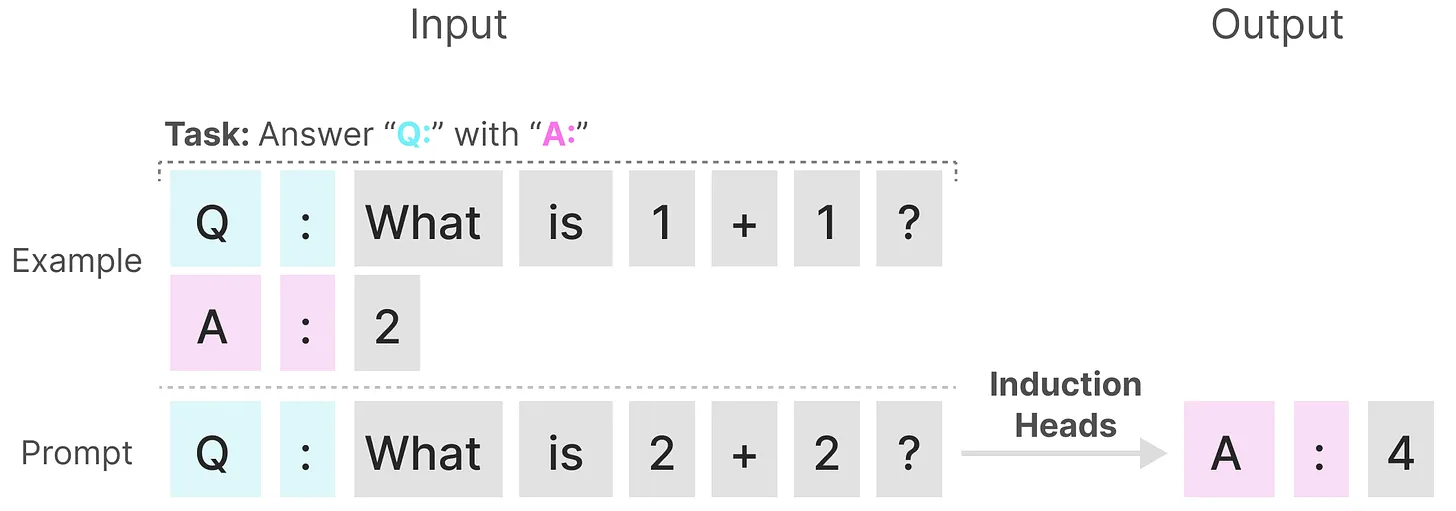
In contrast, these tasks are relatively straightforward for Transformers, as they can dynamically adjust their attention based on the input sequence. This allows them to selectively attend to different parts of the sequence as needed. And the poor performance of SSMs on these tasks highlights the fundamental issue with time-invariant SSMs—the static nature of the matrices $\mathbf{A}$, $\mathbf{B}$, and $\mathbf{C}$ hinders their ability to achieve content-awareness.
Selective SSM (S6)
Compared to S4, the Selective SSM (S6) introduces dynamic behavior by making matrices $\mathbf{B}$ and $\mathbf{C}$, as well as the step size $\Delta t$, dependent on the input by incorporating the sequence length and batch size of the input. Matrix $\mathbf{A}$ remains fixed because the state itself is intended to remain static, while the way it is influenced (through $\mathbf{B}$ and $\mathbf{C}$) to better adapt to varying inputs.
\[\begin{aligned} \mathbf{A} & = \{ A_{ii} \}_{i=1}^N \textrm{ (diagonal) } \in \mathbf{R}^{D \times N = N \times N} \\ \mathbf{B} & = \mathbf{W}_\mathbf{B} \mathbf{x} \in \mathbb{R}^{B \times L \times N} \\ \mathbf{C} & = \mathbf{W}_\mathbf{C} \mathbf{x} \in \mathbb{R}^{B \times L \times N} \\ \Delta & = \texttt{softplus} \left( \Delta t + \texttt{broadcast}_{D} \left(\mathbf{W}_\Delta \mathbf{x} \right) \right) \in \mathbb{R}^{B \times L \times D} \\ \end{aligned}\]where the batched input $\mathbf{x} \in \mathbb{R}^{B \times L \times D}$, projection matrices \(\mathbf{W}_\mathbf{B}, \mathbf{W}_\mathbf{C} \in \mathbb{R}^{B \times L \times N \times D}\) and \(\mathbf{W}_\Delta \in \mathbb{R}^{B \times L \times R \times D}\) such that $R \ll D$. Note that we set $N = D$. With $\Delta$, Mamba uses Zero-Order Hold (ZOH) discretization, which
\[\begin{aligned} & h(t + \Delta) = \exp\left(\Delta \cdot \mathbf{A} \right) h(t) + x(t+1) \int_t^{t+\Delta} \exp \left((t+\Delta-\tau) \cdot \mathbf{A} \right) \mathbf{B} \; \mathrm{d} \tau \\ \Rightarrow & \; \begin{aligned}[t] \bar{\mathbf{A}} & = \exp \left( \Delta \cdot \mathbf{A} \right) \\ \bar{\mathbf{B}} & = \left( \Delta \cdot \mathbf{A} \right)^{−1} \left( \exp \left( \Delta \cdot \mathbf{A} \right) - \mathbf{I} \right) \cdot \Delta \cdot \mathbf{B} \end{aligned} \end{aligned}\]In the practical implementation, the authors slightly simplifies the form of $\bar{\mathbf{B}}$ without affecting empirical performance by Euler method:
\[\bar{\mathbf{B}} \approx \Delta \cdot \mathbf{B}\]which can be justified by the first-order Taylor approximation when $\Delta \cdot \mathbf{A}_{ii} \ll 0$:
\[\left((\Delta \cdot \mathbf{A})^{-1}(\exp \left(\Delta \cdot \mathbf{A} \right)- \mathbf{I})\right)_{ii}=\frac{\exp \left(\Delta \cdot \mathbf{A}_{ii}\right) - 1}{\Delta \mathbf{A}_{ii}} \approx 1\]The following figure summarizes the main algorithmic difference between S4 and S6:
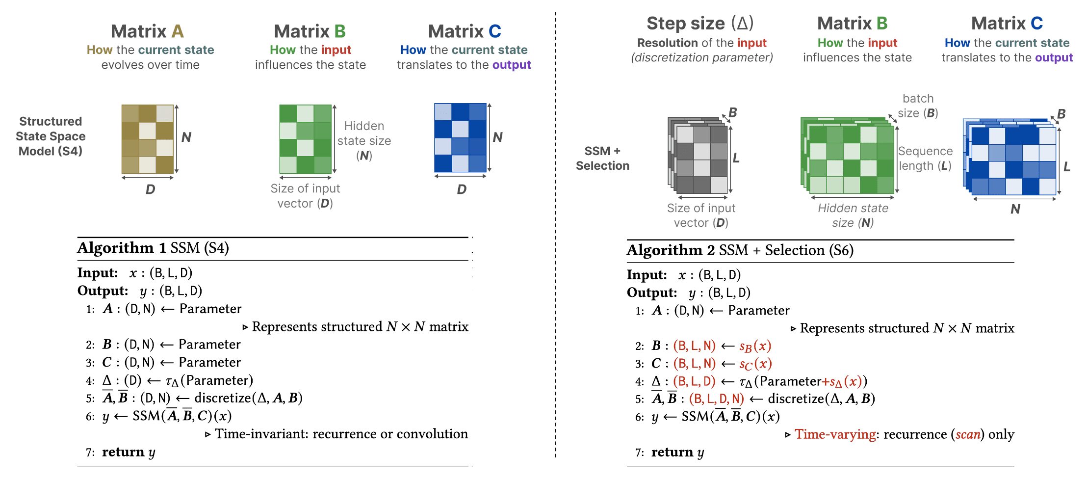
Together, these dynamic adjustments allow S6 to selectively determine what to retain in the hidden state and what to disregard, as they now depend on the input. More broadly, the step size $\Delta$ in SSMs can be viewed as playing a generalized role similar to the gating mechanism in RNNs. For intuition, consider the simplest case of an SSM with $N = 1$, $\mathbf{A} = −1$, $\mathbf{B} = 1$:
\[h(t) = - h(t) + x(t)\]Applying the ZOH discretization formulas, we obtain:
\[\begin{aligned} \bar{\mathbf{A}}_t & = \exp \left( \Delta \cdot \mathbf{A} \right) = \frac{1}{1 + \exp \left( \mathbf{W}_\Delta x_t \right)} \\ & = 1 - \sigma \left( \mathbf{W}_\Delta x_t \right) \\ \bar{\mathbf{B}}_t & = \left(\Delta \cdot \mathbf{A} \right) \left( \exp \left(\Delta \cdot \mathbf{A} \right) - \mathbf{I} \right) \cdot \Delta \cdot \mathbf{B} = - \left( \exp \left(\Delta \cdot \mathbf{A} \right) - \mathbf{I} \right) = 1 - \bar{\mathbf{A}} \\ & = \sigma \left( \mathbf{W}_\Delta x_t \right) \end{aligned}\]Here, a smaller step size $\Delta$ (i.e., smaller $\mathbf{W}_\Delta x_t$) results in relying more on the previous context and ignoring specific words, while a larger step size $\Delta$ emphasizes the input words over the context.
Hardware-Aware Selective Scan Algorithm
Scan operation
Since these matrices are now dynamic, they cannot be calculated using the convolution representation of SSMs since it assumes a fixed kernel. We can only use the recurrent representation and lose the parallelization the convolution provides. To avoid the sequential recurrence, Mamba optimizes its computation using parallel scan algorithm called Blelloch scan algorithm to calculate all-prefix-sums operation in a parallel way:
\[\begin{gathered} \left[\mathbf{A}_0, \mathbf{A}_1, \cdots, \mathbf{A}_{n-1}\right] \\ \Downarrow \\ [\mathbf{0}, \mathbf{A}_0, \left( \mathbf{A}_0 \oplus \mathbf{A}_1 \right), \cdots, \left( \mathbf{A}_0 \oplus \mathbf{A}_1 \oplus \cdots \oplus \mathbf{A}_{n-1} \right)] \end{gathered}\]where $\oplus$ is a binary associative operator (i.e., $(x \oplus y) \oplus z = x \oplus (y \oplus z)$ ).
A parallel computation is work-efficient if it performs asymptotically no more work (in terms of operations, such as additions) than its sequential counterpart. In other words, both the sequential and parallel implementations should have the same work complexity, $\mathcal{O}(n)$. The parallel scan algorithm preserves this overall complexity of $\mathcal{O}(n)$, but by parallelizing the work with $t$ workers, each is responsible for $\mathcal{O}(n/t)$ operations, making the approach efficient overall.
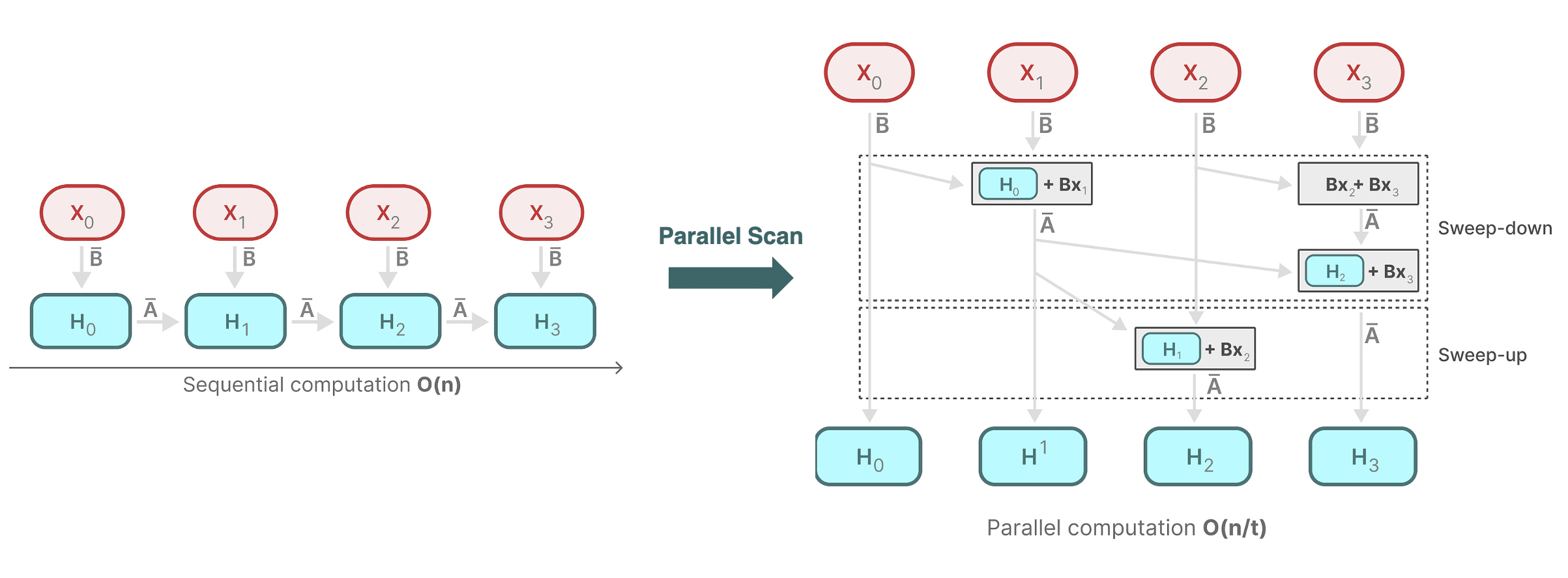
The Blelloch parallel scan consists of two primary operations called up-sweep and down-sweep. The following diagram illustrates the computation process:
- Up-sweep (Reduction Phase)
Compute the parallel reduction of $[\mathbf{A}_0, \cdots, \mathbf{A}_{n-1}]$ that outputs $\mathbf{A}_0 \oplus \mathbf{A}_1 \oplus \cdots \oplus \mathbf{A}_{n-1}$ by constructing a balanced binary tree over the input data. And the algorithm sweeps from the leaves to the root, storing the intermediate results in the corresponding node of the tree at each level. - Down-sweep (Prefix-sum Phase)
Traverse the constructed tree from the root to the leaves, filling in the values with the following rules at any particular node $N$:-
downsweep[N].left.value = downsweep[N].value
The left child's value is set to the current node's value. (A blue node indicates the contribution from the parent.) -
downsweep[N].right.value = downsweep[N].value + upsweep[N].left.value
The right child’s value is the sum of the current node's value and the left child’s value from the up-sweep phase. (A red node indicates a contribution from the downsweep tree, and the yellow node indicates the contribution from the upsweep tree, and orange indicates the combined result.)
-
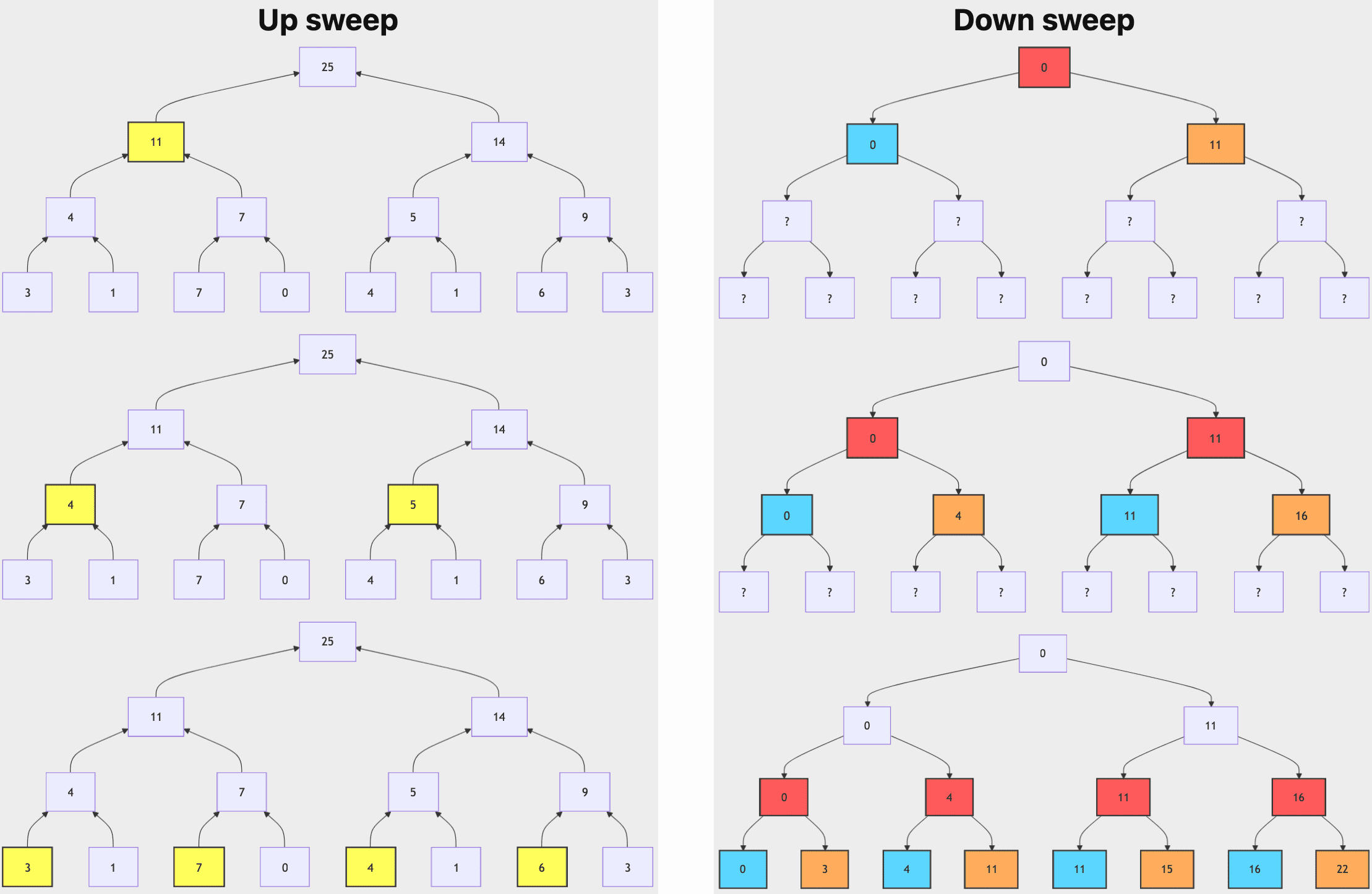
These operations all involve a single traversal of the tree, and therefore require $\mathcal{O}(n)$ operations, as a binary tree with $n$ leaves has $d = \log_2 n$ levels, with each level $d$ containing $2^d$ nodes. Comprehensively, the dynamic matrices $\mathbf{B}$ and $\mathbf{C}$, and the parallel scan algorithm form the selective scan algorithm to represent the dynamic and efficient nature of using the recurrent representations.
Hardware-aware algorithm
Modern GPUs are composed of multiple Streaming Multiprocessors (SMs), alongside an on-chip L2 cache, and high-bandwidth DRAM, commonly known as VRAM, which is specially designed for GPU use. Each SM typically contains additional cores and specialized units, including L1 caches (often referred to as SRAM or shared memory) and registers. SRAM serves as a small, fast memory, positioned close to the SM cores to store frequently accessed data and instructions, thereby minimizing access latency. Registers, which are ultra-fast storage locations within each SM, are dedicated to storing temporary data for active threads, enabling swift access during computation.
Leveraging the distinct characteristics of memory, arithmetic and other instructions are executed by the SMs with the aid of efficient SRAM, while larger data—such as model parameters—and code are accessed from DRAM via the intermediate L2 cache.

However, the limited transfer speed between SRAM and DRAM leads to bottlenecks, particularly during frequent data exchanges. To address this, Mamba reduces transfer between DRAM and SRAM through kernel fusion, a technique that merges multiple operations into a single kernel or function. By reducing the necessity for data transfers between different computation stages, which typically require one DRAM read and one DRAM write per operation, kernel fusion minimizes data movement and memory access, thereby enhancing overall performance.
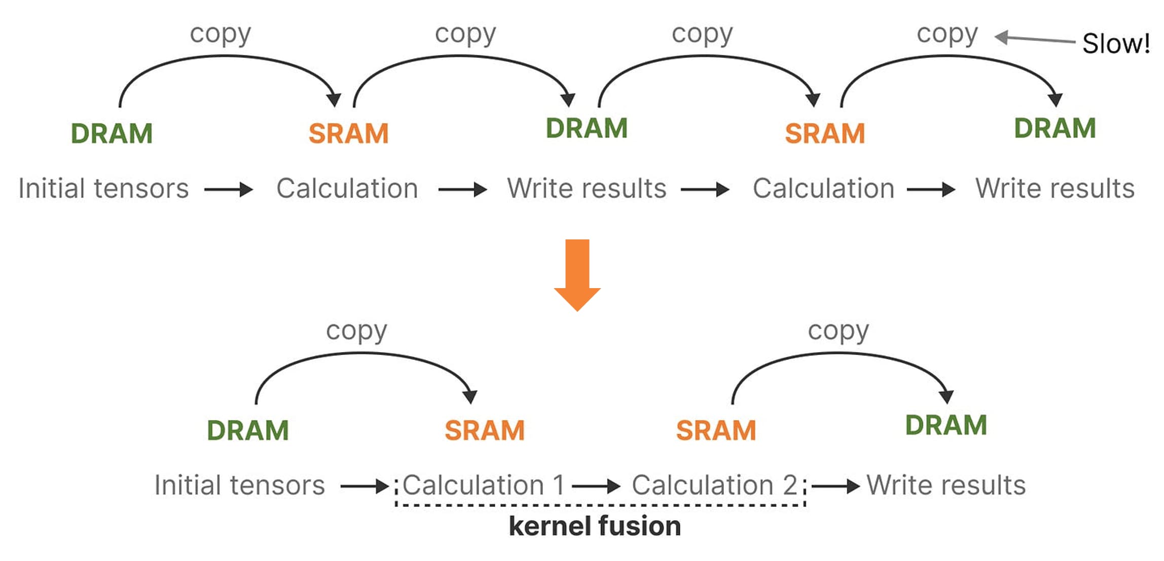
Specifically, in selective SSMs, DRAM stores parameters and SRAM maintains state for fast access. By fusing kernels, Mamba can achieve $7 \times$ faster execution than attention module and improved memory efficiency comparable to FlashAttention, making it a crucial optimization technique. Comprehensively, the overall architecture of a selective SSM or S6 (S4 with the selective scan algorithm) model is illustrated in the following figure:

The Mamba Block
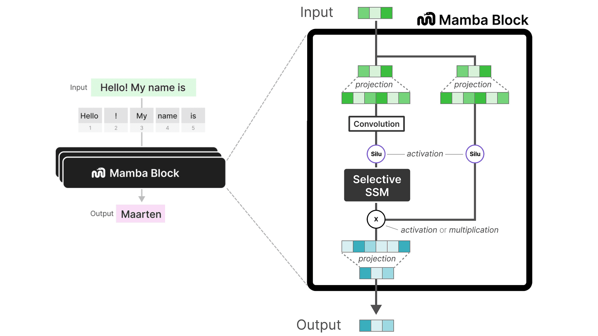
The following figure presents the Mamba block architecture. Within this block, the selective SSM functions as the core component, analogous to the self-attention module in a Transformer block. The process begins with a linear projection to expand the input embeddings, followed by a 1D convolution step. This is done prior to applying the selective SSM, which ensures that token calculations are not performed independently.
References
[1] Gu et al., “HiPPO: Recurrent Memory with Optimal Polynomial Projections”, NeurIPS 2020
[2] T. S. Chihara. An introduction to orthogonal polynomials. Dover Books on Mathematics. Dover Publications, 2011. ISBN 9780486479293.
[3] Gu et al., “LSSL: Combining Recurrent, Convolutional, and Continuous-time Models with Linear State-Space Layers”, NeurIPS 2021
[4] Gu et al., “S4: Efficiently Modeling Long Sequences with Structured State Spaces”, ICLR 2022
[5] Sasha Rush and Sidd Karamcheti, “The Annotated S4”
[6] Gu et al., “Mamba: Efficiently Modeling Long Sequences with Structured State Spaces”, arXiv:2312.00752
[7] Maarten Grootendorst, “A Visual Guide to Mamba and State Space Models”
[8] James Chen, “”
[9] NVIDIA GPU Gems 3 Developers’ Note, “Chapter 39. Parallel Prefix Sum (Scan) with CUDA”
[10] StackOverflow, “CUDA How Does Kernel Fusion Improve Performance on Memory Bound Applications on the GPU?”

Leave a comment