
[Generative Model] Autoregressive Models
By the chain rule of probability, we can factorize the joint distribution over $T$ variable as follows:
This is called an autoregressive model (ARM). The word autoregressive comes from the literature on time-series models, in which predictions of current values are made using data from past time steps’ observations.

$\mathbf{Fig\ 1.}$ Auto-regressive model
But, as the degree of connectivity increases, the required number of parameter for modeling \(p(\mathbf{x}_t \mid \mathbf{x}_{1:t-1})\) tends to increase. To mitigate this inefficiency, one possible way is Markov assumption that simplifies these connectivity:
With this assumption,
\[\begin{aligned} p(\mathbf{x}_{1: T}) = p(\mathbf{x}_1) p(\mathbf{x}_2 \mid \mathbf{x}_1) p(\mathbf{x}_3 \mid \mathbf{x}_2) \cdots = p(\mathbf{x}_1) \prod_{t=2}^T p(\mathbf{x}_t \mid \mathbf{x}_{t-1}) \end{aligned}\]which is called a Markov chain, Markov model, or autoregressive model of order 1. Or, we can make this strong assumption a little weaker by increasing the memory length, and it is called an $M$‘th order Markov model, or $M$-gram model:
Instead of additional assumption, we may maintain the general AR model, but with a restricted form for the conditionals \(p(\mathbf{x}_t \mid \mathbf{x}_{1:t-1})\) that makes the model be easy to compute and optimize. And obviously, the conditional probability can be modeled by deep neural network.
Neural Auto-regressive Density Estimator (NADE)
Neural auto-regressive density estimator (NADE), proposed by Uria et al. 2016, models the conditional probability using neural network.
Assume that the dimensions of $\mathbf{x} = (x_1, \dots, x_D)$ are binary, i.e. \(x_d \in \{0, 1 \}\) for $d = 1, \dots, D$. Then, NADE parameterizes conditional \(p (x_d \mid \mathbf{d}_{< d})\) by feed-forward neural network:
\[\begin{aligned} p (x_d \mid \mathbf{d}_{< d}) & = \sigma(\mathbf{V}_{d, \cdot} \; \mathbf{h}_d + b_d) \\ & = \sigma(\mathbf{V}_{d, \cdot} \; \sigma(\mathbf{W}_{\cdot, < d} \; \mathbf{x}_{< d} + \mathbf{c}) + b_d) \end{aligned}\]where $H$ is the number of hidden units, $\sigma$ stands for sigmoid function, and $\mathbf{V} \in \mathbb{R}^{D \times H}$, $\mathbf{b} \in \mathbb{R}^D$, $\mathbf{W} \in \mathbb{R}^{H \times D}$, $\mathbf{c} \in \mathbb{R}^H$ are the parameters of feed-forward networks i.e. parameters of the NADE model. But hidden layer parameters $\mathbf{W}$ and $\mathbf{c}$ are shared by each hidden layer $\mathbf{h}_d$ for $d = 1, \dots, D$. The following figure illustrates NADE model.
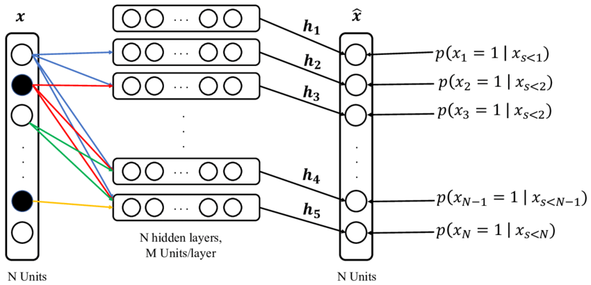
$\mathbf{Fig\ 2.}$ NADE model (source)
In this illustration, units with value 0 are shown in black while units with value 1 are shown in white. The outputs $\widehat{\mathbf{x}}$ correspond to the prediction of conditional probabilities for each dimension of a vector $\mathbf{x}$, given elements earlier to it. And the neural network can be trained in unsupervised way via maximum likelihood (equivalently by minimizing NLL loss):
\[\begin{aligned} \frac{1}{N} \sum_{n=1}^N - \text{ log } p(\mathbf{x}^{(n)}) = \frac{1}{N} \sum_{n=1}^N \sum_{d=1}^D - \text{ log } p(x_d^{(n)} \mid \mathbf{x}_{< d}^{(n)}) \end{aligned}\]And this framework can be naturally extends for non-binary case. If we let \(p(x_t \mid \mathbf{x}_{1:t-1})\) be a conditional mixture of Gaussian, it is known as Real-valued NADE (RNADE) proposed in the same paper with NADE.
\[\begin{aligned} p(x_t \mid \mathbf{x}_{1:t-1}) = \sum_{k=1}^K \pi_{t, k} \mathcal{N}(x_t \mid \mu_{t, k}, \sigma^2_{t, k}) \end{aligned}\]where the parameters for Gaussians mixture are predicted by neural network \((\boldsymbol{\mu}_t, \boldsymbol{\sigma}_t, \boldsymbol{\pi}_t) = f_t (\mathbf{x}_{1 : t-1}; \boldsymbol{\theta}_t)\).
Causal CNNs
Further natural question is whether convolutional neural network can be also employed for modelling \(p( x_t \mid \mathbf{x}_{1 : t-1})\), since it is often powerful to detect some patterns in data.
However, we need to force them to not violate the auto-regressive assumption that the prediction of $x_t$ should depend on past inputs $x_1, \cdots, x_{t - 1}$ only. This can be implemented by masked convolution, also referred to as causal convolution.
For images, causal convolution can be implemented by masking its kernel. But 1-D data such as audio one can more easily implement this by shifting the output of a normal convolution by a few timesteps:
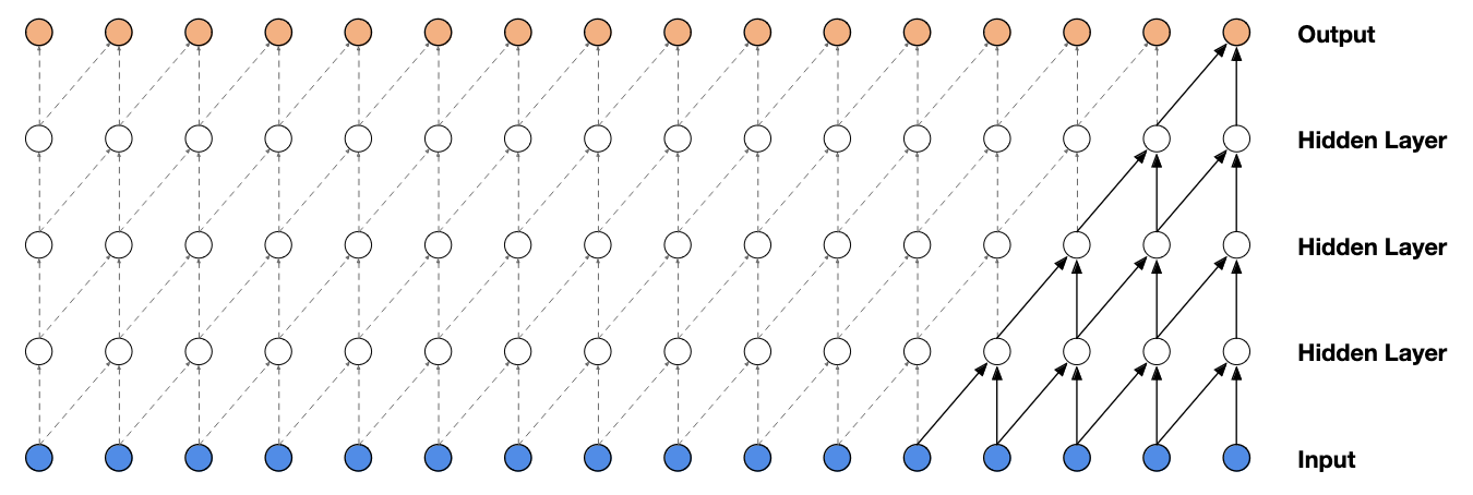
$\mathbf{Fig\ 3.}$ Visualization of a stack of causal convolutional layers. (source: Oord et al. 2016)
1D Causal CNN
For 1D sequences of data $\mathbf{x}_{1:T}$ such as audio and text, the conditional probability can be modeled by 1D causal CNN:
\[\begin{aligned} p(\mathbf{x}_{1:T}) = \prod_{t=1}^T p(x_t \mid \mathbf{x}_{1:t-1}; \Theta) = \prod_{t=1}^T \text{Cat}(x_t \mid \text{softmax}(\sigma) (\sum_{\tau=1}^{t - k} \mathbf{w}^\top \mathbf{x}_{\tau: \tau + k})) \end{aligned}\]where $\mathbf{w} \in \mathbb{R}^k$ is a kernel of 1D CNN, $\sigma$ stands for a non-linearity. (For simplicity, I assumed a single layer of CNN but it can be also much deeper.) Note that it is just 1D convolution, but masked out inputs above $x_t$.
WaveNet ([5]), one of the state-of-the-art text-to-speech generative model, is a representative example of 1D Causal CNN. So as to capture longer range of dependencies without introducing additional parameters, it employed dilated casual convolution:
$\mathbf{Fig\ 4.}$ Visualization of WaveNet using dilated causal convolutions. (source: Oord et al. 2016)
2D Causal CNN: PixelCNN
1D Causal CNN can be naturally extended to 2 dimensional input $\mathbf{x} \in \mathbb{R}^{H \times W}$:
\[\begin{aligned} p(\mathbf{x} \mid \boldsymbol{\theta}) & = \prod_{h=1}^H \prod_{w=1}^W p (x_{r, c} \mid \mathbf{x}_{1:h-1, 1:C}, \mathbf{x}_{r, 1:c-1}) \\ & = \prod_{h=1}^H \prod_{w=1}^W p_{\boldsymbol{\theta}} (x \mid \mathbf{x}_{1:h-1, 1:C}, \mathbf{x}_{r, 1:c-1}) \end{aligned}\]where $p_{\boldsymbol{\theta}}$ is modeled by deep convolutional neural network with softmax. And it is referred to as PixelCNN. Notice that the kernel of network slides in a raster scan order.
![]()
$\mathbf{Fig\ 5.}$ Visualization of PixelCNN
One issue of 2D case is the presence of channel dimension due to RGB pixel values. But it can be mitigated by sequential prediction of pixel value for each channel, in the order of Red-Green-Blue. More formally, for a pixel $x_t = (\color{red}{x_{i, R}}, \color{green}{x_{i, G}}, \color{blue}{x_{i, B}})$:
\[\begin{aligned} p(x_t \mid \mathbf{x}_{1:t-1}) = p(\color{red}{x_{i, R}} \mid \mathbf{x}_{1:t-1}) p(\color{green}{x_{i, G}} \mid \mathbf{x}_{1:t-1}, \color{red}{x_{i, R}}) p(\color{blue}{x_{i, B}} \mid \mathbf{x}_{1:t-1}, \color{red}{x_{i, R}}, \color{green}{x_{i, G}}) \end{aligned}\]
$\mathbf{Fig\ 6.}$ Sequential prediction of RGB
Masked convolution in PixelCNN
For masked convolution, PixelCNN takes two types of masks:
-
Mask A
- only for the first convolutional layer
- allows the model to see previously generated pixels only
- $\therefore$ preserves the causality
-
Mask B
- for all the subsequent convolutional layers
- allows taking value of a pixel currently being predicted into prediction
- it doesn't harm the causality due to mask A
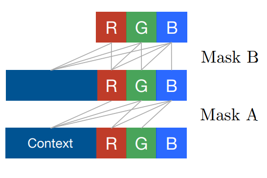
$\mathbf{Fig\ 7.}$ Two types of masks in PixelCNN
PixelCNN Architecture
Finally, the architecture of CNN for PixelCNN is as follows.
![]()
$\mathbf{Fig\ 7.}$ Architecture of PixelCNN (source: current author)
Since the model only takes convolution operations, it is possible to parallelize the model in training time. (But not in generation time, due to the complete past prediction must be needed for each prediction)
Limitation: Blind Spot
Although PixelCNN outperforms image generation models studied at the time, the main drawback is presence of blind spot, arised from the causality. Since the kernel is slid in a raster scan order, the dependency of a pixel, i.e. a receptive field of a pixel tends to be biased towards upper left-side of the image. Hence, this yields large portion of pixels in right-side of input image that can not be considered in prediction:
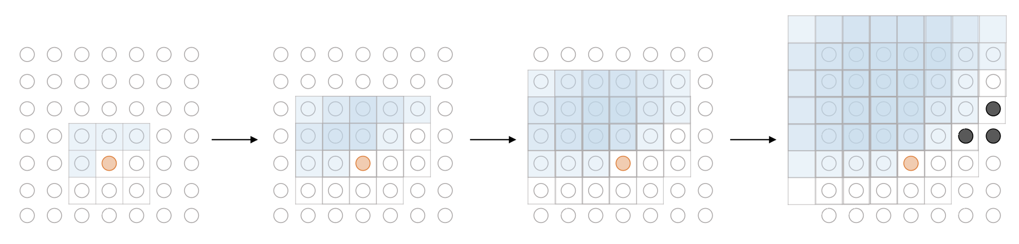
$\mathbf{Fig\ 8.}$ Blind spot (black dots) of PixelCNN
Gated PixelCNN (Oord et al. NeurIPS 2016) removes the blind spot by combining two convolutional network stacks: one that conditions on the current row so far (horizontal stack) and one that conditions on all rows above (vertical stack):
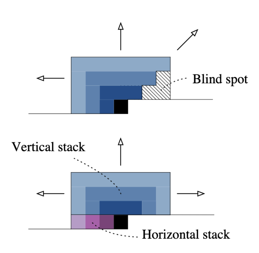
$\mathbf{Fig\ 9.}$ Two orthogonal stacks of conditions (source: Oord et al. NeurIPS 2016)
PixelRNN
For wide range of dependency, PixelCNN must stack convolutional layer much deeper, since the size of receptive field increases linearly. To capture longer range contextual dependencies, PixelRNN combined causal CNN with RNN or LSTM. As a result, although RNN slows down the speed of model, it outperforms PixelCNN with larger dependency range.
(WIP)
PixelTransformer
WIP
Summary
We end this post by summarizing pros and cons of auto-regressive models.
The main advantage of auto-regressive models is that it is conceptually very simple, and easy to optimize and generate. And remarkably, it is able to provide full distribution with probability. But sequential generation is inherently slow, especially for large data, and cannot be parallelized.
Reference
[1] Stanford CS231n, Deep Learning for Computer Vision.
[2] Kevin P. Murphy, Probabilistic Machine Learning: Advanced Topics, MIT Press 2022.
[3] UC Berkeley CS182: Deep Learning, Lecture 17 by Sergey Levine
[4] Uria, Benigno, et al. “Neural autoregressive distribution estimation.” The Journal of Machine Learning Research 17.1 (2016): 7184-7220.
[5] Oord, Aaron van den, et al. “Wavenet: A generative model for raw audio.” arXiv preprint arXiv:1609.03499 (2016).
[6] Van Den Oord, Aäron, Nal Kalchbrenner, and Koray Kavukcuoglu. “Pixel recurrent neural networks.” International conference on machine learning. PMLR, 2016.
[7] Van den Oord, Aaron, et al. “Conditional image generation with pixelcnn decoders.” Advances in neural information processing systems 29 (2016).
Leave a comment