[Generative Model] Variational Autoencoder

Autoencoder

Autoencoder is an unsupervised model for learning feature vectors $z$ from the raw input data $x$ without any labels which is implemented by neural networks. Features should extract useful information of inputs like object identities, properties, and scene type that we can use it for downstream tasks.

Then, how can we extract a feature without any help from supervision (label)? How can we learn this feature transform from raw data? The answer is, use the features to reconstruct the input $\mathbf{\widetilde{x}}$ with a decoder. We train both encoder and decoder with reconstruction error $\sim | | \widetilde{x} - x | |$, and after training, throw away decoder and use encoder for a downstream task.

$\mathbf{Fig\ 1.}$ Illustration of AE

Variational Autoencoder

Introduction

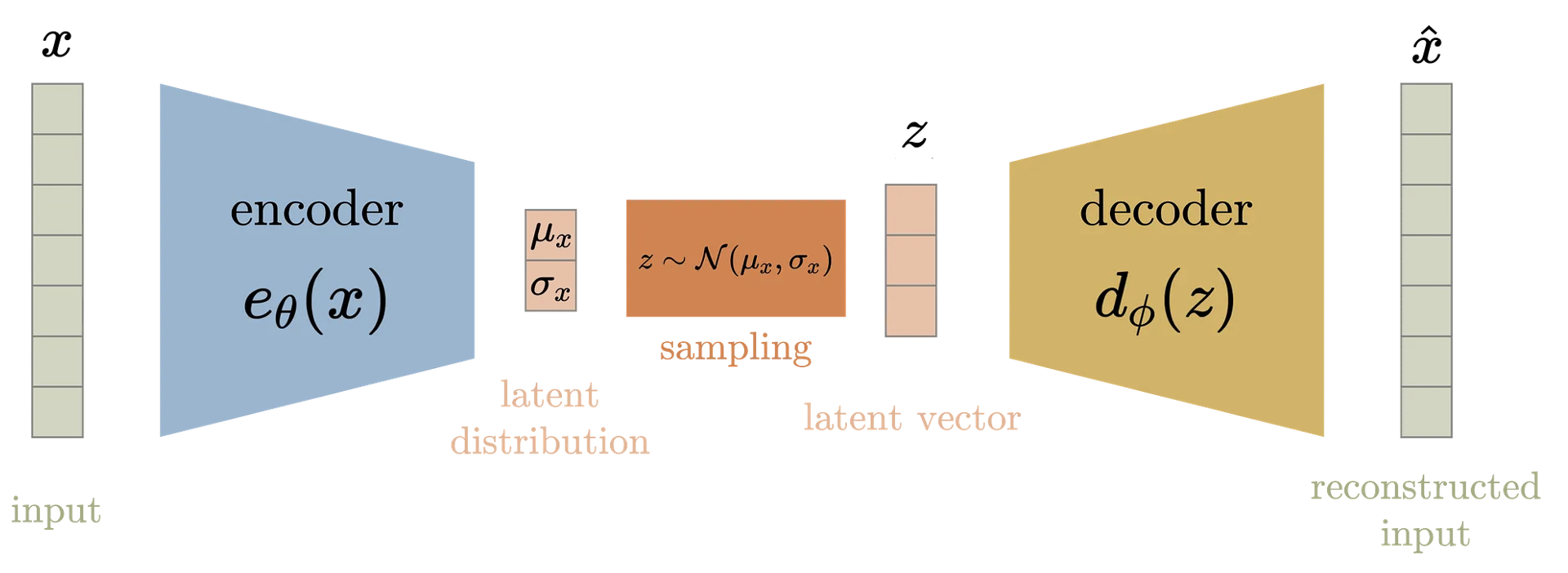
Variational Autoencoder is a probabilistic version of autoencoder, which allows it to sample new data from trained model. The latent space is represented by the probability distribution, and decoder receives as inpput sampled from the latent space and generate a new data similar to the encoder of input $x$.

$\mathbf{Fig\ 2.}$ Illustration of VAE

In contrast to autoencoder, variational autoencoder focuses on the decoder. With an inductive bias that latent space may exists some lower dimension than observation space, variational autoencoder construct a latent space by encoder, and generate new samples.

$\mathbf{Fig\ 3.}$ Latent space exists some lower dimension

Formulation

Let $p_\theta (x) = p(x \mid \theta)$ be the probability distribution of input data $x$, where $\theta$ is the parameter of model. And we should train the model, i.e. find the best parameter $\widehat{\theta}$ that fits the observed dataset distribution. One way to measure the similarity of two distributions is KL divergence:

\[\begin{aligned} \widehat{\theta} = \underset{\theta}{\text{arg min }} \text{KL} (p_{\text{data}} (x) \; \| \; p_\theta (x)) = \mathbb{E}_{x \sim p_{\text{data}}} \left[ \text{ln} \frac{p_{\text{data}} (x)}{p_\theta (x)} \right] \end{aligned}\]

Since $p_{\text{data}}$ is independent of $\theta$, the following optimization problem turns into maximum likelihood estimation that maximizes

\[\begin{aligned} p_\theta (x) = \int p(z) \; p_{\theta} (x \mid z) \; dz \end{aligned}\]

Here, we usually assumes the prior $p (z) \sim \mathcal{N}(\mathbf{0}, \mathbb{I})$ for simplicity, and $p_{\theta} (x | z)$ is a decoder distribution by a deep neural network that takes $z$ as input and outputs an image $x$. Also, it is usually taken to be also Gaussian distribution, e.g. $p_{\theta} (x \mid z) \sim \mathcal{N}(x \mid \mu_{\text{NN}} (z; \; \theta), \sigma^2)$.

Recap: ELBO

Unfortunately, the marginalization is expensive and intractable in most cases. Another idea is Bayes’ rule:

\[\begin{aligned} p_\theta (x) = \frac{p_{\theta} (x \mid z) \; p(z)}{p_{\theta} (z \mid x)} \end{aligned}\]

However, in this case the posterior $p_{\theta} (z \mid x)$ is also intractable generally. So, we should maximize ELBO instead of $p_\theta (x)$ directly. (Note that we cannot apply EM Algorithm which requires the explicit form of $p_{\theta} (z \mid x)$) Recall that ELBO is obtained by:

\[\begin{aligned} \text{ln } p_\theta (x) = F(q, \theta) + \text{KL}(q(z) \; \| \; p_\theta (z \mid x)) \geq F(q, \theta) \end{aligned}\]

where \(F(q, \theta) = \mathbb{E}_{q(z)} \left[ \text{ln } \frac{p_\theta (x,z)}{q(z)} \right]\).

Then, to approximate the integral in expectation, for sampled training data \(\{ x_1, \cdots x_N \}\) and its corresponding latent variables \(\{ z_1, \cdots z_N \}\), $\theta$ is optimized by maximum likelihood estimation with Monte Carlo approximation:

\[\begin{aligned} \widehat{\theta}_{\text{MLE}} & = \underset{\theta}{\text{arg max }} \text{ln } p_\theta (x) \\ & \approx \underset{\theta}{\text{arg max }} F(q, \theta) \\ & \approx \underset{\theta}{\text{arg max }} \frac{1}{N} \sum_{i=1}^N \text{ln } \frac{p_\theta (x_i, z_i)}{q(z_i)} \\ & = \underset{\theta}{\text{arg max }} \frac{1}{N} \sum_{i=1}^N \text{ln } \frac{p_\theta (x_i \mid z_i)}{q(z_i)} \quad \text{ since } \quad p_\theta (x_i) = p ( x_i ) = \mathcal{N}(\mathbf{0}, \mathbb{I}) \end{aligned}\]

And for more expressivity, traditional variational inference usually set $q(z)$ differently for each datapoint $x_i$. It is somewhat intuitive and doesn’t make sense if $q$ has a single parameter, for example $z_i \sim q(z) = \mathcal{N}(\mu, \sigma^2)$ for all $i = 1, \dots, N$, since the behavior of latent variables of individual datapoints may be totally different.

As a result, the number of parameters for training the model is extremely huge if the number of datapoints increases.

Amortized Variational Inference

In addition to decoder network modeling $p_{\theta} (x \mid z)$, VAE introduces the concept of amortization: By introducing the inference network $q_\phi (z \mid x)$, the expensive computational cost of datapoint-wise inference can be amortized.

The additional encoder network $q_\phi (z \mid x)$ parametrized by $\phi$ that approximates the encoder process $p_{\theta} (z \mid x)$. Then, we try to find $\phi$ such that $q_\phi (z \mid x) \approx p_\theta (z \mid x)$ in the sense of minimizing $\text{KL} (q_\phi (z \mid x) \; || \; p_\theta (z \mid x))$.

Then our modified ELBO can be obtained in the same way with ELBO:

\[\begin{aligned} \text{ln } p_\theta (x) &= \mathbb{E}_{q_\phi (z \mid x)} [\text{ln } p_\theta (x)] \\ &= \mathbb{E}_{q_\phi (z \mid x)} \left[\text{ln} \frac{p_\theta (x) p_{\theta} (z \mid x)}{p_{\theta} (z \mid x)} \right] \\ &= \mathbb{E}_{q_\phi (z \mid x)} \left[ \text{ln} \frac{p_\theta (x, z) q_\phi (z \mid x)}{p_{\theta} (z \mid x) q_\phi (z \mid x)} \right] \\ &= \mathbb{E}_{q_\phi (z \mid x)} \left[ \text{ln} \frac{p_\theta (x, z)}{q_\phi (z \mid x)} \right] + \mathbb{E}_{q_\phi (z \mid x)} \left[\text{ln} \frac{q_\phi (z \mid x)}{p_{\theta} (z \mid x)}\right] \\ &\geq \mathbb{E}_{q_\phi (z \mid x)} \left[\text{ln} \frac{p_\theta (x, z)}{q_\phi (z \mid x)} \right] \\ &= \mathbb{E}_{q_\phi (z \mid x)} \left[\text{ln} \frac{p_\theta (x \mid z) p(z)}{q_\phi (z \mid x)} \right] \\ &= \mathbb{E}_{q_\phi (z \mid x)} \left[\text{ln } p_\theta (x \mid z) \right] - \text{KL} (q_\phi (z \mid x) \; \| \; p(z)) \\ &= F(\phi, \theta) \end{aligned}\]

1. Reconstruction term
• $\mathbb{E}_{q_\phi (z \mid x)} \left[\text{ln } p_\theta (x \mid z) \right]$
• encourages that the reconstruction $\widetilde{x}$ is close to the original $x$:
consider a latent vector $z$ that is sampled from the encoder distribution with input data $x$, $q_\phi (z \mid x)$. This reconstruction term is maximized if the decoder distribution from the sampled feature vector $z$ when the input of encoder is data $x$ assigns the high probability mass to the original data $x$. That means, the reconstruction data $\widetilde{x}$ of $x$ will be clustered around the original data $x$.


2. Regularization term
• $\text{KL} (q_\phi (z \mid x) \; \| \; p(z))$
• prevents $q_\phi (z \mid x)$ from moving far away from the prior

Recall that maximizing ELBO with respect to $\phi$ is equivalent to perform approximate posterior inference as $\text{ln } p_\theta (x) = F(\phi, \theta) + \text{KL}(q_\phi (z \mid x) \; || \; p_\theta (z \mid x))$. Since $\mathbf{x}$ is typically much higher dimensional than $\mathbf{z}$, the reconstruction term usually dominates. As a result, if there is a conflict between these two objectives (e.g., due to limited modeling power), the reconstruction accuracy will be favored over posterior inference. Hence the learned posterior may not be a very accurate approximation in that case.

And in VAE, the encoder and decoder network is taken to be

\[\begin{aligned} q_\phi (z \mid x) &= \mathcal{N}(z \mid \mu_\text{NN} (x; \phi), \; \sigma_\text{NN} (x; \phi) \cdot \mathbb{I}) \\ p_\theta (x \mid z) &= \mathcal{N}(x \mid \mu = \widetilde{x}, \; \tau^2) \end{aligned}\]

but also, other distributions like Bernoulli can be selected; it’s totally our choices. Now, we jointly train encoder $q$ and decoder $p$ to maximize $F(\phi, \theta)$!

Training

Learning VAE is gradient-based optimization:

\[\begin{aligned} &\theta \leftarrow \theta + \eta \nabla_\theta F(\phi, \theta) \\ &\phi \leftarrow \phi + \eta \nabla_\phi F(\phi, \theta) \end{aligned}\]

Computing $\nabla_\theta F(\phi, \theta)$ is simple. Since KL term is not dependent on $\theta$, we can ignore it. The gradient of first term can be also approximated by the Monte Carlo method as follows:

\[\begin{aligned} \nabla_\theta \mathbb{E}_{q_\phi (z \mid x)} [\text{ln } p_\theta (x \mid z)] &= \mathbb{E}_{q_\phi (z \mid x)} [\nabla_\theta \text{ ln } p_\theta (x \mid z)] \\ &\approx \nabla_\theta \sum_{s} \text{ ln } p_\theta (x \mid z^{(s)}) \quad \text{ where } \quad z^{(s)} \sim q_\phi (z \mid x) \end{aligned}\]

In contrast, there is an issue when we calculate $\nabla_\phi F(\phi, \theta)$. The second term (KL term) can easily be computed because it is KL divergence between two Gaussians which is analytically computable. In VAE, recall that we use standard Gaussian prior and the approximate posterior is also a Gaussian:

\[\begin{aligned} p(z_i) = \mathcal{N}(0, \mathbb{I}), \quad q_\phi (z_i \mid x_i) = \mathcal{N}( \mu_\phi (x_i), \Sigma_\phi (x_i)) \end{aligned}\]

And KL divergence of two multivariate Gaussians can be computed in closed form, and thus also its gradient.

\[\begin{aligned} &- \text{KL} (q_\phi (z \mid x) \; \| \; p(z)) \\ &= \frac{1}{2} \sum_{d=1}^D (1 + \text{ln}(\sigma_d^2 (x; \phi)) - \mu_d^2(x; \phi) - \sigma_d^2 (x; \phi)) \end{aligned}\]

However, computing the gradient of the first term is somewhat tricky as $z$ is sampled which is not differentiable. Previously, when computing gradient with respect to $\theta$, this was fine because sample $z$ is not dependent on $\theta$ but now $z$ is dependent on $\phi$. It is problematic since random sampling is not a differentiable process. So we cannot backpropagate through sample $z$.

Reparameterization Trick

The key idea to resolve this problem is that a sample from a Gaussian distribution $z \sim \mathcal{N}(\mu_\phi, \sigma^2_\phi)$ can be reparameterized as follows:

\[\begin{aligned} z = \mu_\phi + \sigma_\phi \varepsilon \quad \text{ where } \quad \varepsilon \sim \mathcal{N}(0, 1) \end{aligned}\]

Note that in this form, only $\varepsilon$ is a random sample while $\mu_\phi$ and $\sigma_\phi$ are not. So, as the parameter $\phi$ is dependent only on the mean and the standard deviation but not on $\varepsilon$, it is possible to compute gradient with regard to $\phi$.

Now, we can rewrite the gradient (approximated by Monte Carlo method) as follows:

\[\begin{aligned} \nabla_\phi \mathbb{E}_{q_\phi (z_i \mid x_i)} [\text{ln } p_\theta (x_i \mid z_i)] & \approx \nabla_\theta \sum_{s} \text{ ln } p_\theta (x \mid z_\phi^{(s)}) \quad \text{ where } \quad z_\phi^{(s)} \sim q_\phi (z \mid x) \\ & = \nabla_\theta \sum_{s} \text{ ln } p_\theta (x \mid \mu_\phi + \sigma_\phi \varepsilon^{(s)}) \quad \text{ where } \quad \varepsilon^{(s)} \sim \mathcal{N}(0, 1) \end{aligned}\]

The following figure shows the effect of reparametrization to the architecture of VAE:

$\mathbf{Fig\ 4.}$ Reparametrization trick in VAE (source)

Summary

In summary,

• prior: $p(z) \sim \mathcal{N}(0, \mathbb{I})$
• encoder: $q_\phi (z_i \mid x_i) = \mathcal{N}( \mu_\phi (x_i), \Sigma_\phi (x_i))$
• decoder: $p_\theta (x_i \mid z_i) = \mathcal{N}( \mu_\theta (x_i), \Sigma_\theta (x_i))$
• objective: $\underset{\theta, \phi}{\text{max}} \frac{1}{N} \sum_{i=1}^N \text{ ln } p_\theta(x_i \mid \mu_{\phi} (x_i) + \varepsilon \sigma_{\phi} (x_i)) - \text{KL} (q_\phi (z \mid x_i) \; || \; p(z))$

$\mathbf{Fig\ 5.}$ Summary of VAE (source: Aqeel Anwar)

Variational autoencoders are very similar to autoencoders, but the principal difference of them is, VAEs are the generative model. VAE can be used to generative model that generates new random data sample since the decoder of VAE is learned to decode random points in the low-dimensional latent space to a data in the high-dimensional observation space. Note that the latent space can be represented as the probability distribution. And it encourages local smoothness to perform image interpolation.

$\mathbf{Fig\ 6.}$ Disentanglement of VAE

Reference

[1] Stanford CS231n, Deep Learning for Computer Vision.
[2] Kevin P. Murphy, Probabilistic Machine Learning: Advanced Topics, MIT Press 2022.
[3] Wikipedia, Variational autoencoder