[Generative Model] Generative Adversarial Networks

Implicit generative models

Until now, we saw the generative models that provide an explicit form of the distribution of an observed data $\mathbf{x}$ such as VAE. In this post, we will see Generative Adversarial Networks (GANs) proposed by Ian Goodfellow et al., which is an implicit generative models that is a probabilistic model without an explicit specifictation of the distribution of observed datas. In contrast to explicit generative models, implicit probabilistic model defines a stochastic procedure to directly generate data without the specification of distributions, likelihoods, or observation models. It is somewhat natural in real-world problems: we cannot model the distribution of climate datas explicitly :)

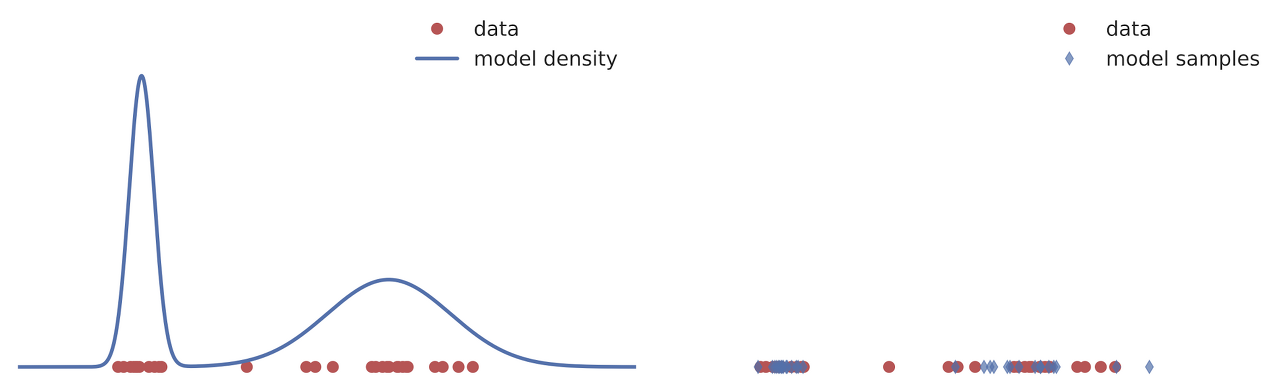
$\mathbf{Fig\ 1.}$ Visualizing the difference between explicit (Left) and implicit generative models (Right).

Training principles of GAN

Note that we cannot evaluate likelihood in implicit models. So, we need another objectives $\mathcal{D}(p^\star, q)$ between the true distribution $p^\star$ and the model $q$ with some nice properties such that

1. It should be minimized when two distributions are same: $$ \begin{aligned} \underset{q}{\text{argmin }} \mathcal{D} (p^\star, q) = p^\star \end{aligned} $$ Or, specifically, like KL divergence, $$ \begin{aligned} \mathcal{D} (p^\star, q) \geq 0; \quad \quad \mathcal{D} (p^\star, q) = 0 \Leftrightarrow q = p^\star \end{aligned} $$
2. It should be tractable only with the observed and generated data
3. Computation should be possible and efficient

But, various distances satisfy the above condition including Wasserstein distance are not comfort to compute or impossible with only using available samples. To overcome this challenges, the main idea of GAN is to approximate the quantity through optimization by introducing a supplemmentary model, discriminator $D$, such that:

\[\begin{aligned} \mathcal{D}(p^\star, q) = \underset{D}{\text{argmax }} \mathcal{F} (D, p^\star, q) \end{aligned}\]

where $\mathcal{F}$ is a functional that depends on $p^\star$ and $q$ only through samples. If we parametrize our distribution estimate $q$ by $\theta$, it is written as

\[\begin{aligned} \mathcal{D}_\phi (p^\star, q) = \underset{\phi}{\text{argmax }} \mathcal{F} (D, p^\star, q_\theta) \end{aligned}\]

To ensure that $\mathcal{F}$ depends on only samples from the model and the unknown data distributon (our second condition for criterion!), the expectations of two distributions can be utilized, which can be Monte-Carlo approximated with only samples:

\[\begin{aligned} \mathcal{F}(\mathcal{D}_\phi, p^\star, q_\theta) = \mathbb{E}_{p^\star(\mathbf{x})} f(\mathbf{x}, \mathbf{\phi}) + \mathbb{E}_{q_\theta (\mathbf{x})} g(\mathbf{x}, \mathbf{\phi}) \end{aligned}\]

Here, the choice of functions $f$ and $g$ totally depend on us, and it determines the form of $\mathcal{F}$. Indeed, the branch of GAN is divided into vanilla GAN, conditional GAN, cycleGAN, etc. according to the choice of $f$ and $g$. We will discuss about them later.

The expression of $\mathcal{F}$ above is the case when estimate distribution $q$ that targets data distribution is parameterized. But in implicit generative models, we cannot model any form to $q_\theta$. Instead, we introduce prior distribution $q$ and latent variable $\mathbf{z} \sim q(\cdot)$ sampled from $q$, and generate the data $\mathbf{x} = G_\theta (\mathbf{z})$ from generative model $G_\theta$ directly. Note that $G_\theta$ is never probability distribution and implicitly model $q_\theta$. In that case, $\mathcal{F}$ can be written in another way:

\[\begin{aligned} \mathcal{F}(\mathcal{D}_\phi, p^\star, q_\theta) = \mathbb{E}_{p^\star(\mathbf{x})} f(\mathbf{x}, \mathbf{\phi}) + \mathbb{E}_{q (\mathbf{z})} g(\mathbf{x} = G_\theta (\mathbf{z}), \mathbf{\phi}) \quad \text{ where } \quad \mathbf{z} \sim q (\mathbf{z}) \end{aligned}\]

Finally, we have to select $f$ and $g$. It is necessary to find a way to properly compare the two distributions $p^\star$ and $q_\theta$. A simple approach to compare them, and also the method used in GAN is the class probability ratio $r( \mathbf{x}) = \frac{p^\star(x)}{q_\theta (x)}$ of the two distributions. And discriminator can be modeled to measure this quantity, e.g. binary classifier $D_\phi (\mathbf{x}) \in [0, 1]$ that input $\mathbf{x}$ is in the class of real data $p^\star$ or generated (fake) data $q_\theta$:

\[\begin{aligned} \frac{p^\star(\mathbf{x})}{q_\theta (\mathbf{x})} = \frac{D_\phi (\mathbf{x})}{1 - D_\phi (\mathbf{x})} \end{aligned}\]

Then, the discriminator can be simply optimized with respect to the parameter $\phi$ via some objective functions like binary cross entropy (BCE) loss. With BCE loss and random variable $y$ for notifying class:

\[\begin{aligned} V(q_\theta, p^\star) & = \underset{\phi}{\text{arg max }} \mathbb{E}_{p(\mathbf{x} \mid y) p(y)} [y \text{ log } D_\phi (\mathbf{x}) + (1 - y) \text{ log } (1 - D_\phi (\mathbf{x}))] \\ & = \underset{\phi}{\text{arg max }} \left\{ \mathbb{E}_{p(\mathbf{x} \mid y=1) p(y=1)} [\text{ log } D_\phi (\mathbf{x})] + \mathbb{E}_{p(\mathbf{x} \mid y=0) p(y=0)} [\text{ log } (1 - D_\phi (\mathbf{x}))] \right\} \\ & = \underset{\phi}{\text{arg max }} \left\{ \mathbb{E}_{p^\star (\mathbf{x})} [\text{ log } D_\phi (\mathbf{x})] + \mathbb{E}_{q_\theta (\mathbf{x})} [\text{ log } (1 - D_\phi (\mathbf{x}))] \right\} \\ & = \underset{\phi}{\text{arg max }} \left\{ \mathbb{E}_{p^\star (\mathbf{x})} [\text{ log } D_\phi (\mathbf{x})] + \mathbb{E}_{q (\mathbf{z})} [\text{ log } (1 - D_\phi (G_\theta (\mathbf{z})))] \right\} \\ \end{aligned}\]

Note that the optimal discriminator $D^\star$ satisfies

\[\begin{aligned} \frac{p^\star(\mathbf{x})}{q_\theta (\mathbf{x})} = \frac{D^\star (\mathbf{x})}{1 - D^\star (\mathbf{x})} \Rightarrow D^\star (\mathbf{x}) = \frac{p^\star (\mathbf{x})}{p^\star (\mathbf{x}) + q_\theta (\mathbf{x})} \end{aligned}\]

By plugging in, we can prove that this objective optimization problem equals to the minimization of Jensen-Shannon divergence (JSD).

\[\begin{aligned} V^\star (q_\theta, p^\star) &= \frac{1}{2} \mathbb{E}_{p^\star (\mathbf{x})} \left[ \text{log } \frac{p^\star (\mathbf{x})}{p^\star (\mathbf{x}) + q_\theta (\mathbf{x})} \right] + \frac{1}{2} \mathbb{E}_{q_\theta (\mathbf{x})} \left[ \text{log } (1 - \frac{p^\star (\mathbf{x})}{p^\star (\mathbf{x}) + q_\theta (\mathbf{x})}) \right] \\ &= \frac{1}{2} \mathbb{E}_{p^\star (\mathbf{x})} \left[ \text{log } \frac{p^\star (\mathbf{x})}{\frac{p^\star (\mathbf{x}) + q_\theta (\mathbf{x})}{2}} \right] + \frac{1}{2} \mathbb{E}_{q_\theta (\mathbf{x})} \left[ \text{log } \frac{q_\theta (\mathbf{x})}{\frac{p^\star (\mathbf{x}) + q_\theta (\mathbf{x})}{2}} \right] - \text{log } 2 \\ &= \frac{1}{2} \text{KL} \left(p^\star \; \| \; \frac{p^\star + q_\theta}{2} \right) + \frac{1}{2} \text{KL} \left(q_\theta \; \| \; \frac{p^\star + q_\theta}{2} \right) - \text{log } 2 \\ &= \text{JSD}(p^\star, q_\theta) - \text{log } 2 \end{aligned}\]

Finally, we can find an optimal parameter $\mathbf{\theta}$ by

\[\begin{aligned} \underset{\mathbf{\theta}}{\text{min }} \text{JSD}(p^\star, q_\theta) &= \underset{\mathbf{\theta}}{\text{min }} \mathbb{E}_{p^\star (\mathbf{x})} [\text{log } D^\star (\mathbf{x})] + \mathbb{E}_{q_\theta (\mathbf{x})} [\text{log } (1 - D^\star (\mathbf{x}))] \\ \end{aligned}\]

Since we don’t know an explicit form of the optimal discriminator $D^\star$, it turns to

\[\begin{aligned} \underset{\mathbf{\theta}}{\text{min }} \text{JSD}(p^\star, q_\theta) &= \left\{ \underset{\mathbf{\theta}}{\text{min }} \underset{\mathbf{\phi}}{\text{max }} \mathbb{E}_{p^\star (\mathbf{x})} [\text{log } D_\mathbf{\phi} (\mathbf{x})] + \mathbb{E}_{q_\theta (\mathbf{x})} [\text{log } (1 - D_\mathbf{\phi} (\mathbf{x}))] \right\} \end{aligned}\]

Lastly, by substituting an explicit generative model $q_\mathbf{\theta}$ for an implicit model $q (\mathbf{z})$ with sampling, it results in

\[\begin{aligned} \underset{\mathbf{\theta}}{\text{min }} \text{JSD}(p^\star, q_\theta) &= \underset{\mathbf{\theta}}{\text{min }} \underset{\mathbf{\phi}}{\text{max }} \mathbb{E}_{p^\star (\mathbf{x})} [\text{log } D_\mathbf{\phi} (\mathbf{x})] + \mathbb{E}_{q (\mathbf{z})} [\text{log } (1 - D_\mathbf{\phi} (\mathbf{x} = G_\mathbf{\theta} (\mathbf{z}) ))] \\ \end{aligned}\]

Although in this post we discuss based on BCE loss (Bernoulli log-loss), other losses are also available; here are some examples.

$\mathbf{Fig\ 2.}$ Examples for loss function

GAN

In the previous section, we look over the basic principles behind the training of GAN. With the understanding of such principle, the architecture and mechanism of GAN can be caught on easily. GANs basically train a discriminator (in this case a binary classifier) only for approximate a divergence between the model and true data distributions. And also, we train the generative model too for minimize this approximation.

From now on, let’s look at the detail of (original) GAN. The full architecture of GAN is as follows:

$\mathbf{Fig\ 3.}$ Full architecture of GAN

Loss functions

The objectives of various type of GANs are formalized as a mini-max game: improve the approximation of the divergence of two distributions and then optimize it, i.e.,

\[\begin{aligned} \underset{\theta}{\text{min }} \underset{\phi}{\text{max }} V(\mathbf{\phi}, \mathbf{\theta}) \end{aligned}\]

where

\[\begin{aligned} V(\mathbf{\phi}, \mathbf{\theta}) = \mathbb{E}_{p^\star (\mathbf{x})} [\text{log } D_\mathbf{\phi} (\mathbf{x})] + \mathbb{E}_{q (\mathbf{z})} [\text{log } (1 - D_\mathbf{\phi} (\mathbf{x} = G_\mathbf{\theta} (\mathbf{z}) ))] \end{aligned}\]

However, in practice such the zero-sum criteria can suffer from the contradiction that the discriminator wants to distinguish between the samples and true datas, whereas the generator tries to generate the indistinguishable sample. Indeed, at start of training, generator performs very bad and discriminator can easily tell apart real and fake, so $D_\phi (G_\mathbf{\theta} (\mathbf{z}))$ close to $0$, which leads to vanishing gradients for generator $G_\mathbf{\theta}$ at the beginning of training:

$\mathbf{Fig\ 4.}$ Plot of $D(G(\mathbf{z}))$ v.s. Generator loss

So, generator instead minimizes

\[\begin{aligned} \underset{\theta}{\text{max }} \mathbb{E}_{q (\mathbf{z})} [- \text{log } D_\mathbf{\phi} (G_\mathbf{\theta} (\mathbf{z}))] \quad \Leftrightarrow \quad \underset{\theta}{\text{min }}\mathbb{E}_{q (\mathbf{z})} [\text{log } (1 - D_\mathbf{\phi}(G_\mathbf{\theta} (\mathbf{z}))) ] \end{aligned}\]

which is known as the nonsaturating loss. It provides better warm-up at the start of the training (strong learning signal when the generative performs badly and the discriminator can easily classify them).

$\mathbf{Fig\ 5.}$ Generator loss and gradient of original loss and non-saturating loss

Based on these, we finally formulate the training losses for the discriminator and generator respectively:

\[\begin{aligned} &L_D (\mathbf{\phi}, \mathbf{\theta}) = \mathbb{E}_{p^\star (\mathbf{x})} [\text{log } D_\mathbf{\phi} (\mathbf{x})] + \mathbb{E}_{q (\mathbf{z})} [\text{log } (1 - D_\mathbf{\phi} ( G_\mathbf{\theta} (\mathbf{z}) ))] \\ &L_G (\mathbf{\phi}, \mathbf{\theta}) = \mathbb{E}_{q (\mathbf{z})} [- \text{log } D_\mathbf{\phi} (G_\mathbf{\theta} (\mathbf{z}))] \end{aligned}\]

Gradient Descent

For training, GAN is optimized by gradient descent for the discriminator and generator. Note that the discriminator allows us to approximate the divergence of two distribution $\mathcal{D}(p^\star, q)$. So, we first train the discriminator and then train the generator in order to minimize the accurate approximation of divergence:

$\mathbf{Fig\ 6.}$ Pseudocode for general GAN training algorithm

For the discriminator $D_\phi$, the gradient with respect to $\phi$ is as follows:

\[\begin{aligned} \nabla_\phi L_D (\mathbf{\phi}, \mathbf{\theta}) = \mathbb{E}_{p^\star (\mathbf{x})} [\nabla_\phi \text{ log } D_\mathbf{\phi} (\mathbf{x})] + \mathbb{E}_{q (\mathbf{z})} [\nabla_\phi \text{ log } (1 - D_\mathbf{\phi} ( G_\mathbf{\theta} (\mathbf{z}) ))] \end{aligned}\]

For the generator $G_\theta$, the gradient with respect to $\theta$ can be computed by reparametrization trick, replace $q$ that allows to change the order of gradient and expectation so that Monte Carlo estimation can be utillized:

\[\begin{aligned} \nabla_\theta L_G (\mathbf{\phi}, \mathbf{\theta}) = \mathbb{E}_{q (\mathbf{z})} [\nabla_\theta - \text{log } D_\mathbf{\phi} (G_\mathbf{\theta} (\mathbf{z}))] \\ \end{aligned}\]

The following figure shows the full training algorithm of GAN proposed in the original paper.

$\mathbf{Fig\ 7.}$ Full training algorithm of GAN proposed in the original paper

cGAN

In an unconditioned generative model, there is no control on modes of the data being generated. cGAN (Mirza et al. 2014), an abbreviation for condition GAN conditions the model on additional information so as to enable the model to direct the data generation process. Such conditioning could be based on class labels, on some part of data for inpainting, or even on data from different modality.

The modification from GAN to cGAN is very simple and straightforward; it performs the conditioning by feeding extra information vector $\mathbf{y}$ into the both the discriminator and generator as additional input layer:

$\mathbf{Fig\ 8.}$ Conditional adversarial net (Mirza et al. 2014)

And the objective function of a minimax game is

\[\begin{aligned} \underset{\text{G}}{\text{min}} \; \underset{\text{D}}{\text{max}} \; V(\text{D}, \text{G}) = \mathbb{E}_{\mathbf{x} \sim p_{\text{data}} (\mathbf{x})} \left[ \text{ log } D( \mathbf{x} \mid \mathbf{y}) \right] + \mathbb{E}_{\mathbf{z} \sim q (\mathbf{z})} \left[ \text{ log } \left(1 - D( G(\mathbf{z} \mid \mathbf{y})) \right) \right] \end{aligned}\]

Hence cGAN can learn conditional distributions of the data $p_{\text{data}}( \mathbf{x} \mid \mathbf{y})$. Here are some conditioned samples in MNIST dataset:

$\mathbf{Fig\ 9.}$ Generated MNIST digits, each row conditioned on one labe (Mirza et al. 2014)

Issues in GAN

Mode collapse and hopping

It is known that the training of GANs is usually suffered from mode collapse. Mode collapse is a phenomenon that the generator underfits to a incomplete distribution which cannot cover not all the modes (peaks) of the data distribution.

Or, it may shows mode hopping that the generator just “hops” between training different modes due to the nature of the mechanism of GAN. Simply, the gerator gives up expanding one mode and jumps to train another mode when the discriminator distinguishes fake datas very well, so that the generator cannot easily generate better one to beat the discriminator and just paves the new way.

Data is a mixture of Gaussians with 16 modes, and the model shows mode collapse and mode hopping.

However, numerous advancements have made GAN training more stable and these behaviors less common. Large batch sizes, regularizations, and more sophisticated optimization techniques are some of these examples.

Reference

[1] Stanford CS231n, Deep Learning for Computer Vision.
[2] Kevin P. Murphy, Probabilistic Machine Learning: Advanced Topics, MIT Press 2022.
[3] Goodfellow, Ian, et al. “Generative adversarial networks.” Communications of the ACM 63.11 (2020): 139-144.
[4] Mirza, Mehdi, and Simon Osindero. “Conditional generative adversarial nets.” arXiv preprint arXiv:1411.1784 (2014).