[Generative Model] Normalizing Flow

GANs and VAEs have outstanding performance on various generative tasks, but some issues limit their application in practice. For example, neither of them do not explicitly model the likelihood function $p_\theta (\mathbf{x})$, which is extremely hard to compute in many cases.

Flow-based generative model is a family of explicit density models with tractable distributions and can explicitly model a probability distribution by leveraging a technique called normalizing flow, popularised by Rezende and Mohamed et al. ICML 2015 in the context of variational inference. A normalizing flow is a transformation of a simple distribution (e.g., Gaussian) into a more complex one by a sequence of invertible and differentiable mappings. As a result, the initial density flows along a sequence of transformations by repeatedly substituting the variable for the new one (mathematically on top of Change of Variables theorem) and obtain a valid probability distribution at the end of the sequence.

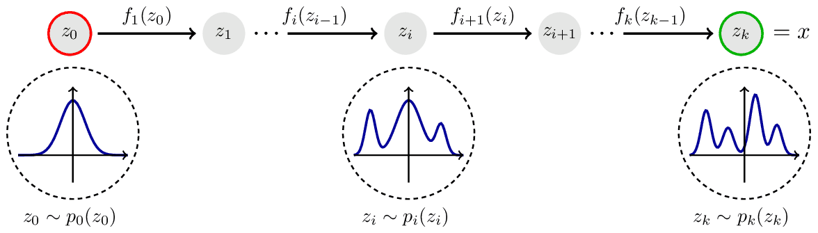
$\mathbf{Fig\ 1.}$ Normalizing Flow (source: TikZ)

Here, the transformation $\mathbf{f}$ pushes forward the base density $p ( \mathbf{z} )$ to a more complex density. Hence, this flow from base density to complex density is referred to as generative direction.

The inverse transformation $\mathbf{f}^{-1}$ flows in the opposite normalizing direction; from complex and irregular data distribution towards the simpler and regular of the base density $p ( \mathbf{z} )$. The term normalizing direction stems from the convention that we usually assumes Gaussian distribution to the prior of latent variable, like in VAE.

Normalizing Flow

Normalizing flows construct complex probability distributions $p(\mathbf{x})$ by passing random variables $\mathbf{z} \in \mathbb{R}^D$, drawn from a simple, and tractable base distribution $p ( \mathbf{z} ): \mathbb{R}^D \to \mathbb{R}$ via a nonlinear invertible transformation $\mathbf{f}: \mathbb{R}^D \to \mathbb{R}^D$. In other words, $p(\mathbf{x})$ is defined & sampled by the following process:

\[\begin{aligned} \mathbf{x} = \mathbf{f}(\mathbf{z}) \quad \text{ where } \quad \mathbf{z} \sim p(\mathbf{z}) \end{aligned}\]

As illustrated in $\mathbf{Fig\ 1.}$, for each iteration $i = 1, \dots, K$, to compute the density $p( \mathbf{x})$

1. Sample $\mathbf{z}_i \sim p_i (\mathbf{z}_i)$
2. Then, it satisfies $\mathbf{z}_{i - 1} = \mathbf{f}_{i}^{-1} (\mathbf{z}_i)$, which normalizes the current distribution by mapping it back to the previous step distribution $p_{i-1}$: $$ \begin{aligned} p_i (\mathbf{z}_i) = p_{i-1}(\mathbf{f}_i^{-1}(\mathbf{z}_i)) \left\vert \det \mathbf{J}_{\mathbf{f}_i^{-1}} (\mathbf{z}_i) \right\vert \end{aligned} $$ where $\mathbf{J}_{\mathbf{f}_i^{-1}} (\mathbf{z}_i)= \frac{\partial \mathbf{f}^{-1}(\mathbf{z}_i)}{\partial \mathbf{z}_i}$ is the Jacobian matrix of $\mathbf{f}_i$ evaluated at $\mathbf{z}_i$.
3. From the inverse function theorem, for $\mathbf{z}_i = \mathbf{f}_i(\mathbf{z}_{i-1})$ and $\mathbf{z}_{i-1} = \mathbf{f}_i^{-1}(\mathbf{z}_i)$ $$ \begin{aligned} \frac{\partial \mathbf{f}_i^{-1}(\mathbf{z}_i)}{\partial \mathbf{z}_i} = \frac{\partial \mathbf{z}_{i - 1}}{\partial \mathbf{z}_i} = \left(\frac{\partial \mathbf{z}_i}{\partial \mathbf{z}_{i-1}} \right)^{-1} = \left( \frac{\partial \mathbf{f}_i(\mathbf{z}_{i-1})}{\partial \mathbf{z}_i} \right)^{-1} \end{aligned} $$ In other words, $\mathbf{J}_{\mathbf{f}_i^{-1}} (\mathbf{z}_i) = \mathbf{J}_{\mathbf{f}_i} (\mathbf{z}_{i-1})^{-1}$ Hence $$ \begin{aligned} p_i (\mathbf{z}_i) = p_{i-1}(\mathbf{f}_i^{-1}(\mathbf{z}_i)) \left\vert \det \mathbf{J}_{\mathbf{f}_i} (\mathbf{z}_{i-1})^{-1} \right\vert = p_{i-1}(\mathbf{z}_{i-1}) \frac{1}{\left\vert \det \mathbf{J}_{\mathbf{f}_i} (\mathbf{z}_{i-1}) \right\vert} \end{aligned} $$

Hence, we can solve this recurrence relation by

\[\begin{aligned} \mathbf{x} = \mathbf{z}_K = \mathbf{f}_K \circ \mathbf{f}_{K-1} \circ \cdots \circ \mathbf{f}_1 (\mathbf{z}_0) \end{aligned}\]

and

\[\begin{aligned} \text{log } p(\mathbf{x}) = \text{ log } p_K (\mathbf{z}_K) & = \text{ log } p_{K-1} (\mathbf{z}_{K-1}) - \text{ log } \left\vert \det \mathbf{J}_{\mathbf{f}_K} (\mathbf{z}_{K-1}) \right\vert \\ & = \text{ log } p_{K-2} (\mathbf{z}_{K-2}) - \text{ log } \left\vert \det \mathbf{J}_{\mathbf{f}_{K-1}} (\mathbf{z}_{K-2}) \right\vert - \text{ log } \left\vert \det \mathbf{J}_{\mathbf{f}_K} (\mathbf{z}_{K-1}) \right\vert \\ & = \cdots \\ & = \text{ log } p_{0} (\mathbf{z}_{0}) - \sum_{i=1}^K \text{ log } \left\vert \det \mathbf{J}_{\mathbf{f}_i} (\mathbf{z}_{i-1}) \right\vert \end{aligned}\]

Thus, the equation implies that if the transformation $\mathbf{f}$ is invertible and has Jacobian determinant that can be computed efficiently, one can construct complex densities $p(\mathbf{x})$.

And, as the exact form of log-likelihood of data is now available, flow-based models can be simply optimized through the NLL loss over the training dataset $\mathcal{D}$:

\[\begin{aligned} \mathcal{L}(\boldsymbol{\theta}) = - \frac{1}{\left\vert \mathcal{D} \right\vert} \sum_{\mathbf{x} \in \mathcal{D}} \text{ log } p_{\boldsymbol{\theta}} (\mathbf{x}) \end{aligned}\]

Various Normalizing Flow model

So in the remaining part of the post, we discuss how to compute and construct various kinds of normalizing flow.

NICE (Dinh et al. ICLRW 2015)

NICE, an abbreviation for Non-linear Independent Component Estimation (Dinh, et al. 2015), propose coupling flows to design $\mathbf{f}$ by feed-forward network in an invertible way.

The authors define an (additive) coupling layer $\mathbf{f}: \mathbf{z} \in \mathbb{R}^\text{D} \mapsto \mathbf{x} \in \mathbb{R}^\text{D}$ as follows:

\[\begin{cases} \mathbf{x}_{1:d} & = \mathbf{z}_{1:d} \\ \mathbf{x}_{d+1: \text{D}} & = \mathbf{z}_{d+1: \text{D}} + \mathbf{f}_{\boldsymbol{\theta}}(\mathbf{z}_{1:d}) \\ \end{cases}\]

for some $1 \leq d \leq \text{D}$ and feed-forward network $\mathbf{f}_{\boldsymbol{\theta}}$. In other words,

\[\begin{aligned} \mathbf{f} (\mathbf{z})_i = \begin{cases} \mathbf{z}_i & \text{ if } \quad 1 \leq i \leq d \\ \mathbf{z}_i + \mathbf{f}_{\boldsymbol{\theta}}(\mathbf{z}_{1:d})_i & \text{ otherwise } \end{cases} \end{aligned}\]

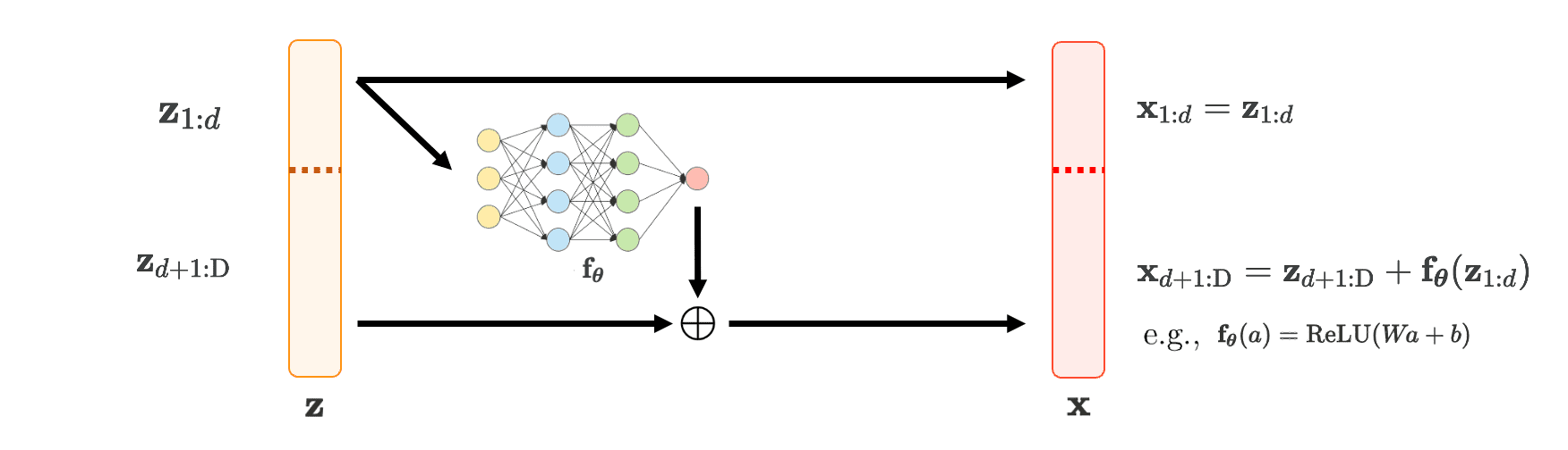
$\mathbf{Fig\ 2.}$ Coupling layer framework (Inspired by Sergey Levine, created by current author)

Then, the transformation $\mathbf{f}$ satisfies some desirable properties that we expect:

Invertible (bijection)

\[\begin{aligned} \mathbf{f}^{-1} (\mathbf{x})_i = \begin{cases} \mathbf{x}_i & \text{ if } \quad 1 \leq i \leq d \\ \mathbf{x}_i - \mathbf{f}_{\boldsymbol{\theta}}(\mathbf{x}_{1:d})_i & \text{ otherwise } \end{cases} \end{aligned}\]

Manageable Jacobian

The Jacobian forms a lower triangular matrix:

\[\begin{aligned} \mathbf{J}_\mathbf{f} = \left[ \begin{array}{c:c} \frac{\partial \mathbf{x}_{1:d}}{\partial \mathbf{z}_{1:d}} & \frac{\partial \mathbf{x}_{1:d}}{\partial \mathbf{z}_{d+1:\text{D}}} \\ \hdashline \frac{\partial \mathbf{x}_{d+1: \text{D}}}{\partial \mathbf{z}_{1:d}} & \frac{\partial \mathbf{x}_{d+1: \text{D}}}{\partial \mathbf{z}_{d+1:\text{D}}} \end{array} \right] = \left[ \begin{array}{c:c} \mathbb{I}_d & \mathbf{0}_{d \times (\text{D} - d)} \\ \hdashline \frac{\partial \mathbf{f}_{\boldsymbol{\theta}}}{\partial \mathbf{z}_{1:d}} & \mathbb{I}_{\text{D} - d} \end{array} \right] \end{aligned}\]

which is comfortable to compute determinant and inverse matrix. And it doesn’t involve \(\mathbf{f}_{\boldsymbol{\theta}}\) in calculation of inverse transformation or determinant of Jacobian, we are free to design arbitrarily model for \(\mathbf{f}_{\boldsymbol{\theta}}\).

However, as determinant of Jacobian is always 1, it doesn’t change the scale, so that it’s representationally a bit limiting.

Result

As a result, NICE generates quite natural images for simple data distribution such as MNIST. But in case of complicated distributions such as human face, we can observe that the generated samples are noisy and low-quality.

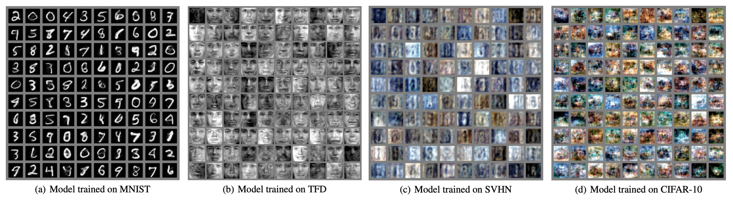
$\mathbf{Fig\ 3.}$ Samples of NICE (source: Dinh et al. ICLRW 2015)

Real-NVP (Dinh et al. ICLR 2016)

Real-NVP: Non-Volume Preserving Transformatio (Dinh, et al. ICLR 2016) is a subsequent work of NICE. It slightly modified the operation of additive coupling layer:

\[\begin{cases} \mathbf{x}_{1:d} &= \mathbf{z}_{1:d} \\ \mathbf{x}_{d+1: \text{D}} &= \mathbf{z}_{d+1: \text{D}} \odot \text{exp} (\mathbf{s}_{\boldsymbol{\theta}} (\mathbf{x}_{1:d})) + \mathbf{t}_{\boldsymbol{\phi}} (\mathbf{x}_{1:d}) \end{cases}\]

where \(\mathbf{s}_{\boldsymbol{\theta}}\) and \(\mathbf{t}_{\boldsymbol{\phi}}\) are neural networks for scaling and translation respectively. Notice that we take an exponential of scale function to prevent multiplying zero that destroys invertibility. And this modified version of additive coupling layer is referred to as affine coupling layer.

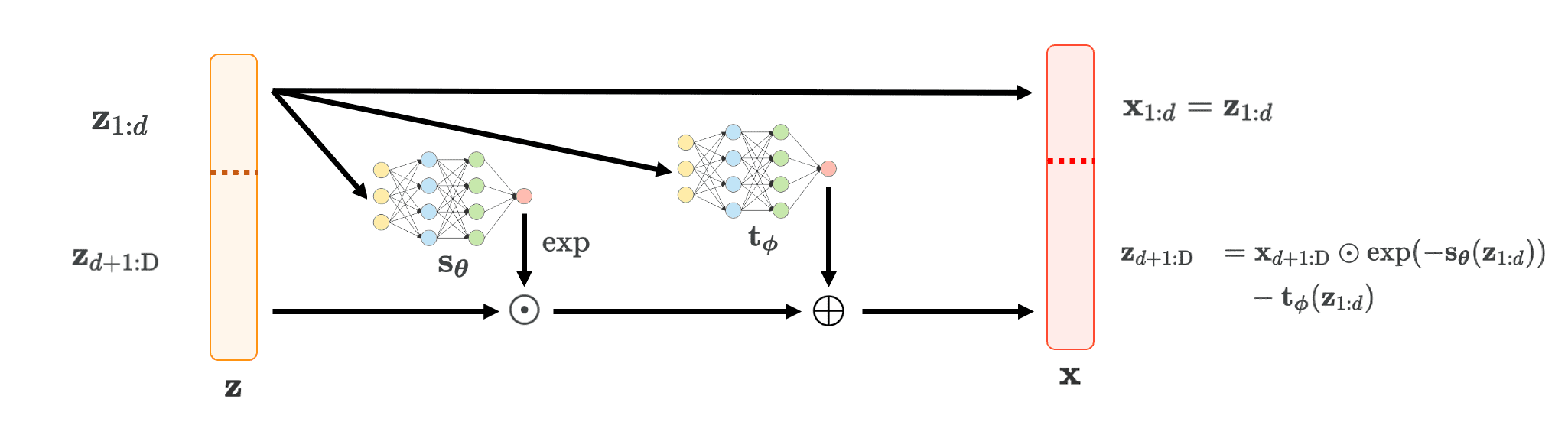
$\mathbf{Fig\ 4.}$ Affine coupling layer framework (Inspired by Sergey Levine, created by current author)

Invertible (bijection)

\[\begin{cases} \mathbf{z}_{1:d} & = \mathbf{x}_{1:d} \\ \mathbf{z}_{d+1:\text{D}} & = \mathbf{x}_{d+1:\text{D}} \odot \text{exp} (-\mathbf{s}_{\boldsymbol{\theta}} (\mathbf{z}_{1:d})) - \mathbf{t}_{\boldsymbol{\phi}} (\mathbf{z}_{1:d}) \end{cases}\]

Manageable Jacobian

The Jacobian forms a lower triangular matrix:

\[\begin{aligned} \mathbf{J}_\mathbf{f} = \left[ \begin{array}{c:c} \frac{\partial \mathbf{x}_{1:d}}{\partial \mathbf{z}_{1:d}} & \frac{\partial \mathbf{x}_{1:d}}{\partial \mathbf{z}_{d+1:\text{D}}} \\ \hdashline \frac{\partial \mathbf{x}_{d+1: \text{D}}}{\partial \mathbf{z}_{1:d}} & \frac{\partial \mathbf{x}_{d+1: \text{D}}}{\partial \mathbf{z}_{d+1:\text{D}}} \end{array} \right] = \left[ \begin{array}{c:c} \mathbb{I}_d & \mathbf{0}_{d \times (\text{D} - d)} \\ \hdashline \frac{\partial \mathbf{x}_{d+1: \text{D}}}{\partial \mathbf{z}_{1:d}} & \text{exp} (\mathbf{s}_{\boldsymbol{\theta}} (\mathbf{x}_{1:d})) \odot \mathbb{I}_{D-d} \end{array} \right] \end{aligned}\]

Then, determinant of Jacobian can be efficiently computed:

\[\begin{aligned} \text{det}(\mathbf{J}_\mathbf{f}) = \prod_{i=1}^{\text{D}-d} \text{exp} (\mathbf{s}_{\boldsymbol{\theta}} (\mathbf{x}_{1:d}))_i = \text{exp} \left( \sum_{i=1}^{\text{D} - d} \mathbf{s}_{\boldsymbol{\theta}} (\mathbf{x}_{1:d})_i \right) \end{aligned}\]

hence it is significantly expressive than NICE modeling:

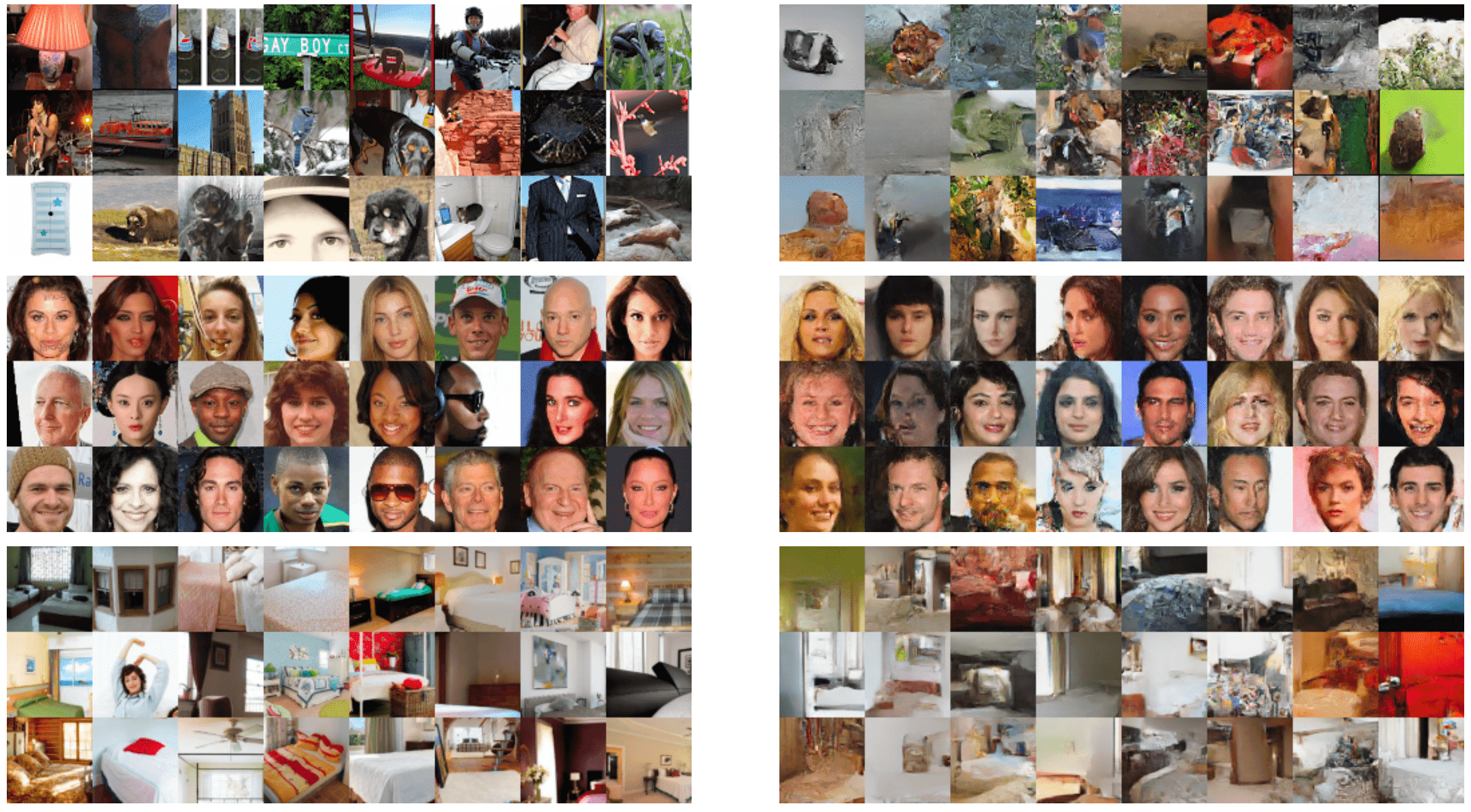
$\mathbf{Fig\ 5.}$ Samples of Real-NVP (Left: examples in dataset, Right: generated samples) (source: Dinh et al. ICLR 2016)

Reference

[1] Stanford CS236, Deep Generative Models.
[2] Kevin P. Murphy, Probabilistic Machine Learning: Advanced Topics, MIT Press 2022.
[3] GitHub, Awesome Normalizing Flows
[4] D. J. Rezende and S. Mohamed, “Variational Inference withNormalizing Flows,” in ICML, 2015.
[5] Papamakarios, George, et al. “Normalizing flows for probabilistic modeling and inference.” The Journal of Machine Learning Research 22.1 (2021): 2617-2680.
[6] Dinh, Laurent, David Krueger, and Yoshua Bengio. “Nice: Non-linear independent components estimation.” arXiv preprint arXiv:1410.8516 (2014).
[7] Dinh, Laurent, Jascha Sohl-Dickstein, and Samy Bengio. “Density estimation using Real NVP.” International Conference on Learning Representations. 2016.