[Generative Model] VQ-VAE

Introduction

Despite the challenges associated with using discrete latent variables in deep learning, vector quantizing VAE (VQ-VAE) proposed by Van Den Oord et al. 2017 differentiably combines the VAE framework with discrete latent representations. The model is built on vector quantization (VQ) method, which maps $K$-dimensional vectors into a finite set of code vectors maintained in codebooks.

$\mathbf{Fig\ 1.}$ VQ-VAE framework (Van Den Oord et al. NeurIPS 2017)

VQ-VAE

Forward computation pipeline

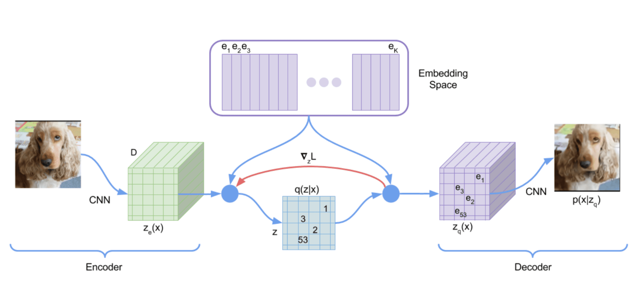
Define a latent embedding space $\mathbf{e} \in \mathbb{R}^{K \times D}$, where $K$ is the size of the discrete latent space (i.e., a $K$-way categorical), and $D$ is the dimensionality of each latent embedding vector $\mathbf{e}_i$. Then, the forward computation of VQ-VAE operates as following:

1. An image input $\mathbf{x}$ is passed through an encoder $f_\theta$, producing output $f_\theta (\mathbf{x}) \in \mathbb{R}^D$. For brevity, assume $\mathbf{x} \in \mathbb{R}^N$ is one-dimensional vector.
2. The discrete latent variables $\mathbf{z}$ are then calculated by nearest neighbor look-up of the shared embedding space $\mathbf{e}$: $$ k = \arg \min_j \lVert f_\theta (\mathbf{x}) - \mathbf{e}_j \rVert_2 $$ Hence the posterior categorical distribution $q(\mathbf{z} \vert \mathbf{x})$ probabilities are defined as one-hot as follows: $$ \begin{aligned} q(\mathbf{z} = k \vert \mathbf{x}) = \begin{cases} 1 & \quad \text{for } k = \arg \min_j \arg \min_j \lVert f_\theta (\mathbf{x}) - \mathbf{e}_j \rVert_2 \\ 0 & \quad \text{ otherwise } \end{cases} \end{aligned} $$
3. The input $\mathbf{z}_\mathbf{q} (\mathbf{x})$ to the decoder $g_\phi$ is the corresponding embedding vector $\mathbf{e}_k$: $$ \begin{aligned} \mathbf{z}_\mathbf{q} (\mathbf{x}) = \mathbf{e}_k \quad \text{ where } \quad k = \arg \min_j \lVert f_\theta (\mathbf{x}) - \mathbf{e}_j \rVert_2 \end{aligned} $$

Although the above discussion is using an one-dimensional $\mathbf{x}$ and a single random variable $\mathbf{z}$ to represent the discrete latent variables, but it can be generalized to 2D matrix and tensors.

Training Loss

The training loss $\mathcal{L}$ has 3 components:

1. Reconstruction Loss
   From the reconstructed data $\tilde{\mathbf{x}} \sim p (\cdot \vert \mathbf{z}_\mathbf{q} (\mathbf{x}))$ from decoder output $\mathbf{z}_\mathbf{q} (\mathbf{x})$, the reconstruction loss encourages that the reconstruction $\tilde{\mathbf{x}}$ is close to the original $\mathbf{x}$: $$ \mathcal{L}_\texttt{recon} = \log p (\mathbf{x} \vert \mathbf{z}_\mathbf{q} (\mathbf{x})) $$ which is equivalent to $\ell_2$ loss $\Vert g_\phi (\mathbf{z}_\mathbf{q} (\mathbf{x})) - \mathbf{x} \Vert_2^2$ if the decoder distribution $p$ is set to be Gaussian distribution. Additionally, since the $\arg \min$ operator is not differentiable, the gradients $\nabla_\mathbf{z} \mathcal{L}$ from decoder input $\mathbf{z}_\mathbf{q} (\mathbf{x})$ is copied to the encoder output $f_\theta (\mathbf{x})$, which is called straight-through gradient estimation.
2. Vector Quantization Loss
   To learn embedding space $\mathbf{e}$, the vector quantization (VQ) loss is defined as $\ell_2$ error between the embedding space and the encoder outputs. Given a code vector $\mathbf{e}_i$, let $\{ \mathbf{z}_{i, j} \}_{j=1}^{n_i}$ be the set of encoder output vectors $f_\theta (\mathbf{x})$ that are quantized to $\mathbf{e}_i$. Then, the loss term is given by: $$ \mathcal{L}_{\texttt{VQ}} = \sum_{j=1}^{n_i} \Vert \texttt{stopgrad} ( \mathbf{z}_{i, j} ) - \mathbf{e}_i \Vert_2^2 $$ Note that it has a closed form solution (the average of elements in the set): $$ \mathbf{e}_i^* = \frac{1}{n_i} \sum_{j=1}^{n_i} \mathbf{z}_{i, j} $$ Therefore, instead of gradient descent, we can also use this update rule which is typically used in algorithms such as K-Means. However, we cannot use this update directly when working with minibatches since all $\{ \mathbf{z}_{i, } \}_{j=1}^{n_i}$ are not accessible. Instead, the embeddings are updated by exponential moving averages (EMA) as an online version of this update: $$ \begin{aligned} N_i^{(t)} & := \gamma N_{i}^{(t-1)} + (1-\gamma)n_i^{(t)} \\ m_i^{(t)} & := \gamma m_{i}^{(t-1)} + (1-\gamma) \sum_{j} z_{i, j}^{(t)} \\ e_i^{(t)} & := \frac{m_i^{(t)}}{N_i^{(t)}} \end{aligned} $$ where $\gamma \in [0, 1]$, and $N_i$ and $m_i$ are accumulated vector count and volume, respectively. (But the authors simply update the codebook with gradient descent in their official implementation, so you can ignore this.)
3. Commitment Loss
   Since there are no constraints on the embedding space, it can grow arbitrarily. A commitment loss, regularization to get encoder outputs and codebook close, is added to the overall loss function: $$ \mathcal{L}_{\texttt{commitment}} = \Vert f_\theta (\mathbf{x}) - \texttt{stopgrad} [ \mathbf{e} = \mathbf{z}_\mathbf{q} (\mathbf{x}) ] \Vert_2^2 $$ which encourages the encoder output $f_\theta (\mathbf{x})$ to stay close to the embedding space $\mathbf{e}$ and to prevent it from fluctuating too frequently from one code vector to another.

The following equation specifies the overall loss function.

\[\begin{aligned} \mathcal{L} & = \underbrace{\log p(\mathbf{x} \vert \mathbf{z}_\mathbf{q} (\mathbf{x}))}_{\textrm{reconstruction loss}} + \underbrace{\lVert \texttt{stopgrad}[\mathbf{z}_\mathbf{e} (\mathbf{x})] - \mathbf{e} \rVert_2^2}_{\textrm{VQ loss}} + \underbrace{\beta \times \lVert \mathbf{z}_\mathbf{e} (\mathbf{x}) - \texttt{stopgrad}[\mathbf{e}]\rVert_2^2}_{\textrm{commitment loss}} \\ & = \Vert g_\phi (\mathbf{z}_\mathbf{q} (\mathbf{x})) - \mathbf{x} \Vert_2^2 + \Vert \texttt{stopgrad} (f_\theta (\mathbf{x})) - \mathbf{z}_\mathbf{q} (\mathbf{x}) \Vert_2^2 + \beta \times \Vert f_\theta (\mathbf{x}) - \texttt{stopgrad} (\mathbf{z}_\mathbf{q} (\mathbf{x})) \Vert_2^2 \end{aligned}\]

where $\texttt{stopgrad}$ is the stop-gradient operator.

Straight-Through Estimator

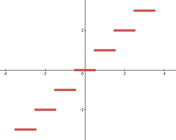
For better understanding of straight-through estimator, let’s consider the following neural network that contains $\texttt{round}()$ function:

import torch
x = torch.tensor([1.1, 2.1], requires_grad=True)
y = 2*x
z = torch.round(y)
r = z.sum()

However, when we try to compute the gradient, we get a tensor of zeroes:

r 
# tensor(6., grad_fn=<SumBackward0>)
r.backward()
x.grad
# tensor([0., 0.])

This is because the rounding function has derivative zero almost everywhere.

$\mathbf{Fig\ 2.}$ The plot of $\texttt{round}$ function

To circumvent non-differentiability, we could simply ignore the rounding function for the backpropagation and forcibly skip the gradient $\partial r \/\partial z = \partial r / \partial y$ in order to maximize/minimize the output $r$:

x = torch.tensor([1.1, 2.1], requires_grad=True)
y = 2*x
z = torch.round(y)
z = y + (z - y).detach() # Detach everything between z and y, including z
r = z.sum()

Then, we get reasonable gradients of $x$ for our objective:

r 
# tensor(6., grad_fn=<SumBackward0>)
r.backward()
x.grad
# tensor([2., 2.])

Prior distribution $p(z)$

While training, the prior distribution over the discrete latents $p(z)$ is a uniform distribution, and can be made autoregressive by depending on other $z$ in the feature map.

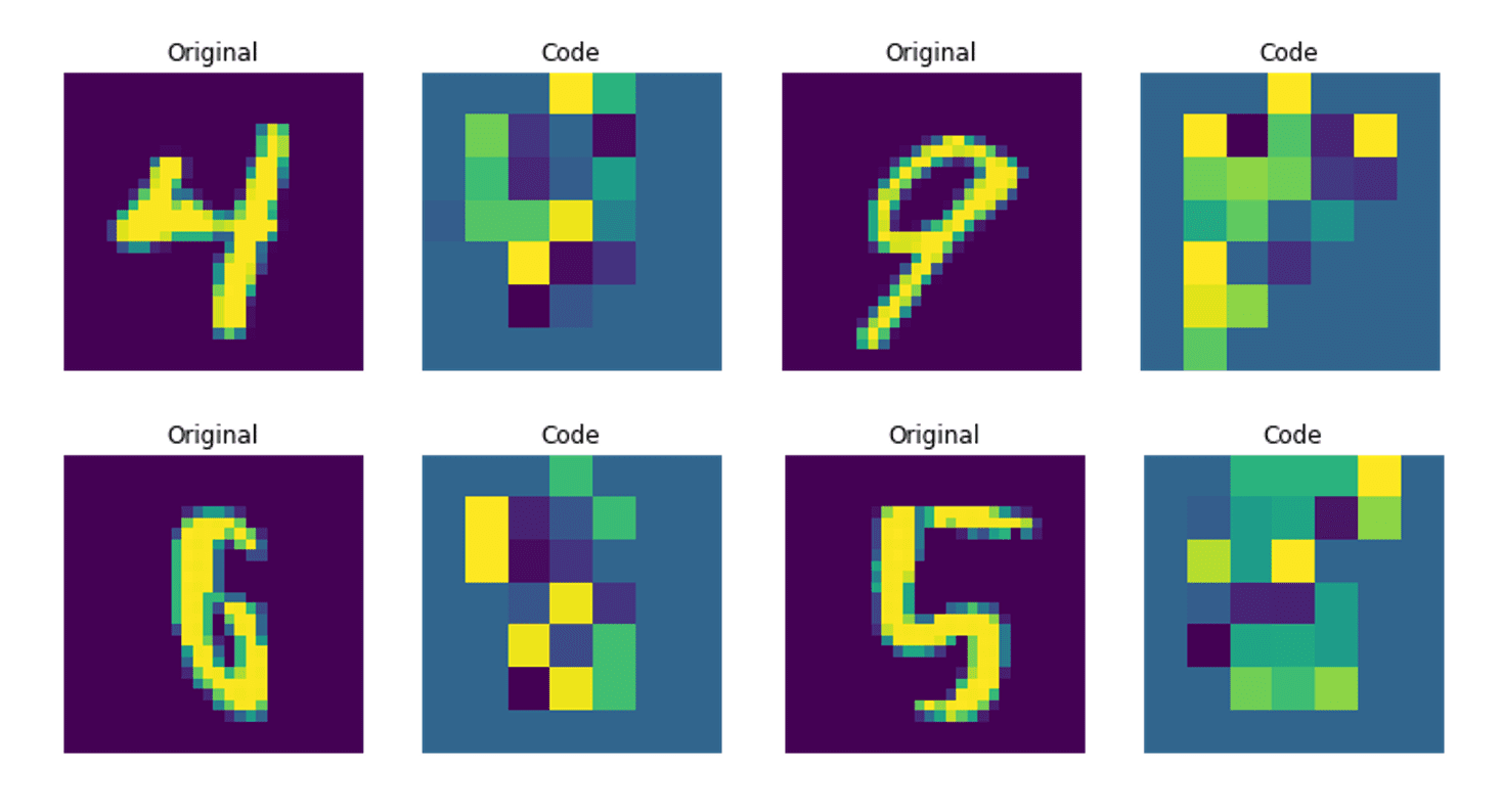
At first, train usual VQ-VAE with uniform prior. The figure below shows that the discrete codes are able to capture some regularities from the MNIST dataset. But since the distribution of the codebook $p(z)$ is simply uniform distribution, this is not enough to generate novel and meaningful images. Not only the form of embedding vectors, but also the relationships (dependencies) between them should be learned for the inference stage.

$\mathbf{Fig\ 3.}$ Trained embedding codes on MNIST dataset (Sayak Paul)

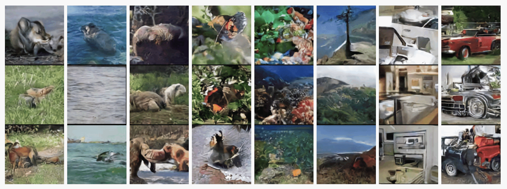
To solve certain problems of uniform initialization of codebook, we freeze VQ-VAE and train autoregressive generative model (e.g. PixelCNN for image tasks, WaveNet for audio tasks) to predict the embedding vector, represented as embedding space indices. Then the trained VQ-VAE decoder is used to map the indices generated by the autoregressive model back into the data space. By coupling these representations with an autoregressive prior, VQ-VAE models can generate high quality samples. Moreover, this enables not only a substantial acceleration of training and sampling but also the utilization of the autoregressive model’s capability to capture the global structure.

$\mathbf{Fig\ 4.}$ Samples (128x128) from a VQ-VAE with a PixelCNN prior trained on ImageNet images. (Van Den Oord et al. NeurIPS 2017)

Reference

[1] Van Den Oord et al. “Neural discrete representation learning.” NeurIPS 2017..
[2] Sayak Paul, Vector-Quantized Variational Autoencoders, Keras