[Generative Model] Score-based Generative Models

Introduction

Score-based models, in particular score-based generative models are built over the technique called score matching. Score matching is originally designed in Hyvärinen et al. JMLR 2005 for learning unnormalized probabilistic model, or energy-based model implicitly (i.e. from an unknown data distribution), but Song and Ermon et al. NeurIPS 2019 repurpose it for generative modeling. Hence to provide motivation for score matching, it is imperative to have a comprehension of energy-based models.

\[\begin{aligned} p_{\theta} (\mathbf{x}) = \frac{e^{-f_\theta (\mathbf{x})}}{Z_\theta}, \end{aligned}\]

where $Z_\theta > 0$ is a normalizing constant to ensure $\int p_{\theta} (\mathbf{x}) \; d\mathbf{x} = 1$. Given a dataset \(\mathcal{D} = \{ \mathbf{x}_{n} \mid n = 1, \cdots N \}\), it is possible to train the model by maximum log-likelihood estimation:

\[\begin{aligned} \hat{\theta} = \underset{\theta}{\operatorname{argmax}} \sum_{n=1}^N \log p_{\theta} ( \mathbf{x}_n ). \end{aligned}\]

The main challenge of this maximum likelihood estimation is, $Z_\theta = \int e^{-f_{\theta}(\mathbf{x})} \; d\mathbf{x}$ is usually not tractable for all general $f_{\theta}(\mathbf{x})$. And in the aftermath of intractability, likelihood-based models must either

• restrict their model architectures,
  • autoregressive models
  • normalizing flow models
• or approximate the normalizing constant
  • VAE

but the computational expense comes at the price. Instead of estimating the density function, score matching aims to learn the score, gradient of log-likelihood defined as

\[\begin{aligned} \nabla_\mathbf{x} \log p (\mathbf{x}) \end{aligned}\]

One should be aware of disparity with score in statistics; score in the jargon of statistics usually refers to the gradient with regard to parameter $\theta$, $\nabla_\theta \log p_{\theta} (\mathbf{x})$, for the purpose of point estimation of unknown parameters. Estimating the gradient of data distribution from the observed sample may still seem to be a very difficult way, since it is basically a non-parametric estimation problem. However, the authors proved that any calculation of such data distribution is not needed. It will be shortly discussed below. Furthermore, it is known that score matching gives exactly the same estimator as maximum likelihood estimation in case of Gaussian parameter estimation. [3]

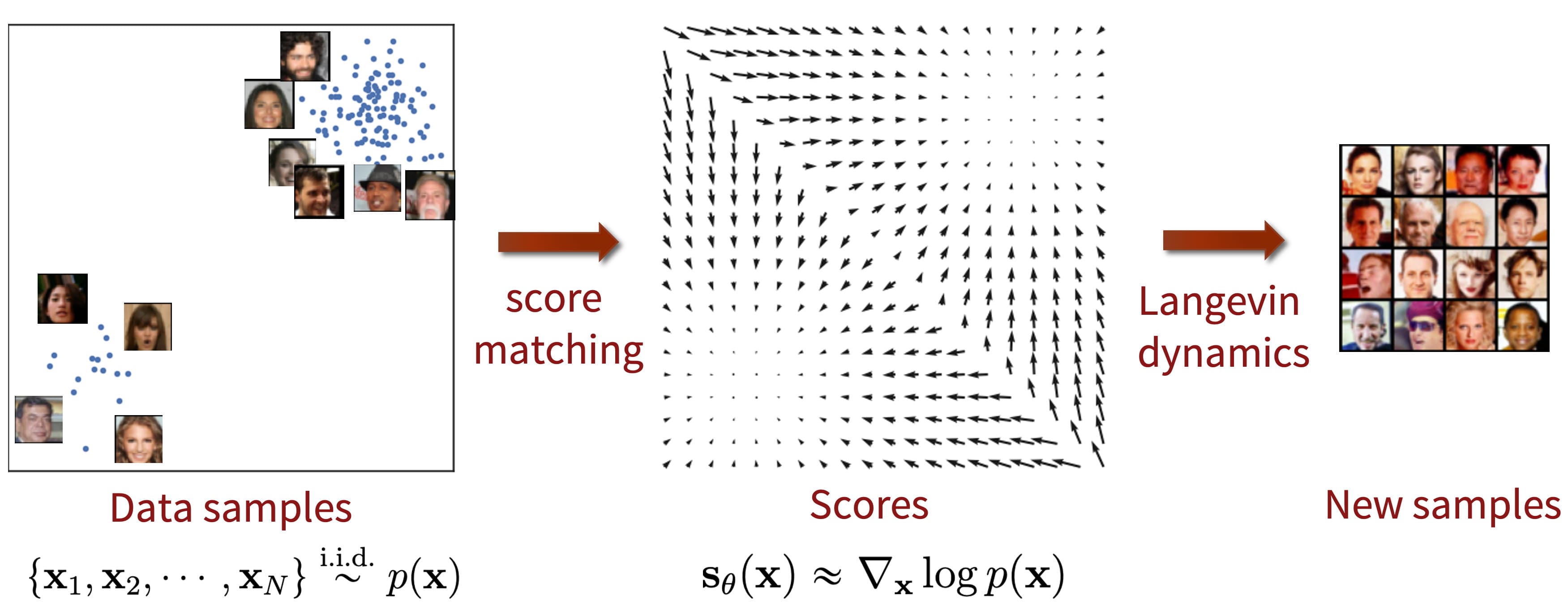
$\mathbf{Fig\ 1.}$ Score-based generative model (source: Yang Song's blog)

In short, there are intrinsic limitations in likelihood-based generative models:

• use specialized architectures to build a normalized probability model
  • autoregressive models
  • flow-based models
• use of surrogate loss
  • e.g. ELBO in VAE

GANs avoid some of the limitations of likelihood-based models, but

• their training can be unstable due to the adversarial training procedure
• the GAN objective is not suitable for evaluating and comparing different GANs

Score-based models is based on estimating and sampling from the score, the gradient of the logarithmic data density, to skirt limitations of likelihood-based models.

Score-based generative modeling

Here are our notations:

• Datapoints: \(\{ \mathbf{x}_i \in \mathbb{R}^{\text{D}} \mid i=1, \cdots N \}\)
• Data distribution: $p_{\text{data}} (\mathbf{x})$
• Score of $p (\mathbf{x})$: $\nabla \text{ log } p (\mathbf{x})$
• Score network $\mathbf{s}_{\boldsymbol{\theta}}: \mathbb{R}^{\text{D}} \to \mathbb{R}^{\text{D}}$
  • It is trained to approximate $\nabla_{\mathbf{x}} \text{ log } p_{\text{data}} (\mathbf{x})$

The framework of score-based generative modeling has two ingredients: score matching and Langevin dynamics.

I. Score matching for score estimation

We directly train \(\mathbf{s}_{\boldsymbol{\theta}} (\mathbf{x})\) to estimate $\nabla_{\mathbf{x}} \text{ log } p_{\text{data}} (\mathbf{x})$ without estimating $p_{\text{data}} (\mathbf{x})$, by minimizing the objective

\[\begin{aligned} J (\boldsymbol{\theta}) = \frac{1}{2} \mathbb{E}_{p_{\text{data}} (\mathbf{x})} \left[ \| \mathbf{s}_{\boldsymbol{\theta}} (\mathbf{x}) - \nabla_{\mathbf{x}} \text{ log } p_{\text{data}} (\mathbf{x}) \|_2^2 \right] \end{aligned}\]

As $\mathbf{s}_{\boldsymbol{\theta}} (\mathbf{x})$ stands for the score, this objective is usually known as Fisher divergence between the model $q$ and the data distributions $p$:

\[\begin{aligned} \mathbb{E}_{p(\mathbf{x})}[\| \nabla_\mathbf{x} \log p(\mathbf{x}) - \nabla_\mathbf{x}\log q(\mathbf{x}) \|_2^2]. \end{aligned}\]

But it is not analytically computable as $p_{\text{data}} (\mathbf{x})$ is unknown in general. Instead, the data distribution can be discarded provided that we assume some regularity condition:

\[\begin{aligned} J (\boldsymbol{\theta}) = \mathbb{E}_{p_{\text{data}} (\mathbf{x})} \left[ \text{tr} (\nabla_{\mathbf{x}} \mathbf{s}_{\boldsymbol{\theta}} (\mathbf{x})) + \frac{1}{2} \| \mathbf{s}_{\boldsymbol{\theta}} (\mathbf{x}) \|_2^2 \right]. \end{aligned}\]

Hyvärinen et al. JMLR 2005, the original paper of score matching, provided the detail of the proposition and proof. (click to expand)

$\color{red}{\mathbf{Theorem.}}$ Suppose

1. the data distribution $p_{\text{data}} (\mathbf{x})$ is differentiable;
2. $\mathbb{E}_{p_{\text{data}}}[\| \mathbf{s}_{\boldsymbol{\theta}} (\mathbf{x}) \|_2^2] < \infty$ for any $\boldsymbol{\theta}$;
3. $\mathbb{E}_{p_{\text{data}}}[\| \nabla_{\mathbf{x}} \text{ log } p_{\text{data}} (\mathbf{x}) \|_2^2] < \infty$;
4. $\lim_{\|\mathbf{x}\| \to \infty} \mathbf{s}_{\boldsymbol{\theta}} (\mathbf{x}) \cdot \nabla_{\mathbf{x}} \text{ log } p_{\text{data}} (\mathbf{x}) = 0$ for any $\boldsymbol{\theta}$.

Then, the optimization problem $$ \begin{aligned} \underset{\boldsymbol{\theta}}{\text{ min }} \frac{1}{2} \mathbb{E}_{p_{\text{data}} (\mathbf{x})} \left[ \| \mathbf{s}_{\boldsymbol{\theta}} (\mathbf{x}) - \nabla_{\mathbf{x}} \text{ log } p_{\text{data}} (\mathbf{x}) \|_2^2 \right] \end{aligned} $$ is equivalent to $$ \begin{aligned} \underset{\boldsymbol{\theta}}{\text{ min }} \mathbb{E}_{p_{\text{data}} (\mathbf{x})} \left[ \text{tr} (\nabla_{\mathbf{x}} \mathbf{s}_{\boldsymbol{\theta}} (\mathbf{x})) + \frac{1}{2} \| \mathbf{s}_{\boldsymbol{\theta}} (\mathbf{x}) \|_2^2 \right]. \end{aligned} $$ Furthermore, let the estimated data distribution with $\boldsymbol{\theta}$ be $p_{\boldsymbol{\theta}} (\mathbf{x})$ and $p_{\text{data}} = p_{\boldsymbol{\theta}^*}$ for some $\boldsymbol{\theta}^*$. If we additionally assume that

5. no other $\boldsymbol{\theta}$ estimates a data distribution that is equal to the estimated data distribution with $\boldsymbol{\theta}^*$;
6. a function $q_{\boldsymbol{\theta}}: \mathbb{R}^{\text{D}} \to \mathbb{R}$ that satisfies $$ \begin{aligned} \mathbf{s}_{\boldsymbol{\theta}} (\mathbf{x}) = \frac{\partial \text{ log } q_{\boldsymbol{\theta}} (\mathbf{x})}{\partial \mathbf{x}} \end{aligned} $$ is greater than $0$ for all $\mathbf{x}, \boldsymbol{\theta}$;

$\boldsymbol{\theta}^*$ is the minimizer of these equations, i.e. satisfies $\mathbf{s}_{\boldsymbol{\theta}^*} (\mathbf{x}) = \nabla_{\mathbf{x}} \text{ log } p_{\text{data}} (\mathbf{x})$ almost everywhere.

$\mathbf{Proof.}$

First, unfold the expectation in $L_2$ loss:

\[\begin{aligned} & \frac{1}{2} \int p_{\text{data}} (\mathbf{x}) \| \mathbf{s}_{\boldsymbol{\theta}} (\mathbf{x}) - \nabla_{\mathbf{x}} \text{ log } p_{\text{data}} (\mathbf{x}) \|_2^2 \; d\mathbf{x} \\ = & \int p_{\text{data}} (\mathbf{x}) \left[ \frac{1}{2} \| \mathbf{s}_{\boldsymbol{\theta}} (\mathbf{x}) \|_2^2 + \frac{1}{2} \| \nabla_{\mathbf{x}} \text{ log } p_{\text{data}} (\mathbf{x}) \|_2^2 - \mathbf{s}_{\boldsymbol{\theta}} (\mathbf{x})^\top \nabla_{\mathbf{x}} \text{ log } p_{\text{data}} (\mathbf{x}) \right] \; d\mathbf{x} \\ \end{aligned}\]

Note that the second term inside the bracket is negligible in terms of optimizing with respect to parameters. Therefore, it suffices to consider

\[\begin{aligned} \int p_{\text{data}} (\mathbf{x}) \left[ - \mathbf{s}_{\boldsymbol{\theta}} (\mathbf{x})^\top \nabla_{\mathbf{x}} \text{ log } p_{\text{data}} (\mathbf{x}) \right] \; d\mathbf{x}. \end{aligned}\]

It equals to

\[\begin{aligned} - \sum_{j=1}^{\text{D}} \int \mathbf{s}_{\boldsymbol{\theta}} (\mathbf{x})_j \frac{\partial p_{\text{data}} (\mathbf{x})}{\partial \mathbf{x}_j} \; d\mathbf{x}. \end{aligned}\]

And each summand satisfies

\[\begin{aligned} \int \mathbf{s}_{\boldsymbol{\theta}} (\mathbf{x})_j \frac{\partial p_{\text{data}} (\mathbf{x})}{\partial \mathbf{x}_j} \; d\mathbf{x} & = \int \left[ \int_{-\infty}^{\infty} \mathbf{s}_{\boldsymbol{\theta}} (\mathbf{x})_j \frac{\partial p_{\text{data}} (\mathbf{x})}{\partial \mathbf{x}_j} \; d\mathbf{x}_j \right] \; d (\mathbf{x}_1 \cdots \mathbf{x}_{j-1} \mathbf{x}_{j+1} \cdots \mathbf{x}_{\text{D}}). \end{aligned}\]

Through integration by parts and assumption at infinities, we have

\[\begin{aligned} & \int_{-\infty}^{\infty} \mathbf{s}_{\boldsymbol{\theta}} (\mathbf{x})_j \frac{\partial p_{\text{data}} (\mathbf{x})}{\partial \mathbf{x}_j} \; d\mathbf{x}_j \\ = & \; \big[ p_{\text{data}} (\mathbf{x}_1, \cdots, \mathbf{x}_j, \cdots, \mathbf{x}_{\text{D}}) \mathbf{s}_{\boldsymbol{\theta}} (\mathbf{x}_1, \cdots, \mathbf{x}_j, \cdots, \mathbf{x}_{\text{D}})_j \big]_{-\infty}^\infty - \int_{-\infty}^\infty p_{\text{data}} (\mathbf{x}) \frac{\partial \mathbf{s}_{\boldsymbol{\theta}} (\mathbf{x})_j}{\partial \mathbf{x}_j} \; d\mathbf{x}_j \\ = & - \int_{-\infty}^\infty p_{\text{data}} (\mathbf{x}) \frac{\partial \mathbf{s}_{\boldsymbol{\theta}} (\mathbf{x})_j}{\partial \mathbf{x}_j} \; d\mathbf{x}_j \end{aligned}\]

Therefore,

\[\begin{aligned} - \sum_{j=1}^{\text{D}} \int \mathbf{s}_{\boldsymbol{\theta}} (\mathbf{x})_j \frac{\partial p_{\text{data}} (\mathbf{x})}{\partial \mathbf{x}_j} \; d\mathbf{x} & = \sum_{j=1}^{\text{D}} \int p_{\text{data}} (\mathbf{x}) \frac{\partial \mathbf{s}_{\boldsymbol{\theta}} (\mathbf{x})_j}{\partial \mathbf{x}_j} \; d\mathbf{x} \\ & = \int p_{\text{data}} (\mathbf{x}) \text{ tr} \left( \nabla_{\mathbf{x}} \mathbf{s}_{\boldsymbol{\theta}} (\mathbf{x}) \right) \; d\mathbf{x} \\ & = \mathbb{E}_{p_{\text{data}} (\mathbf{x})} \left[ \text{tr} \left( \nabla_{\mathbf{x}} \mathbf{s}_{\boldsymbol{\theta}} (\mathbf{x}) \right) \right] \end{aligned}\]

which shows the first statement in the theorem.

For the second statement, it suffices to show that if we set

\[\begin{aligned} J (\boldsymbol{\theta}) = \mathbb{E}_{p_{\text{data}} (\mathbf{x})} \left[ \text{tr} (\nabla_{\mathbf{x}} \mathbf{s}_{\boldsymbol{\theta}} (\mathbf{x})) + \frac{1}{2} \| \mathbf{s}_{\boldsymbol{\theta}} (\mathbf{x}) \|_2^2 \right] + \text{ const. } \\ & = \frac{1}{2} \mathbb{E}_{p_{\text{data}} (\mathbf{x})} \left[ \| \mathbf{s}_{\boldsymbol{\theta}} (\mathbf{x}) - \nabla_{\mathbf{x}} \text{ log } p_{\text{data}} (\mathbf{x}) \|_2^2 \right] \end{aligned}\]

then

\[\begin{aligned} J (\boldsymbol{\theta}^*) = 0 \quad \text{ if and only if } \quad \mathbf{s}_{\boldsymbol{\theta}^*} (\mathbf{x}) = \nabla_{\mathbf{x}} \text{ log } p_{\text{data}} (\mathbf{x}) \text{ a.e. } \end{aligned}\]

For the proof, assume $J (\boldsymbol{\theta}^*) = 0$. Then the assumption 6 implies that $p_{\text{data}} (\mathbf{x}) > 0$ for all $\mathbf{x}$, which implies $\nabla_{\mathbf{x}} \text{ log } p_{\text{data}} (\mathbf{x})$ and $\nabla_{\mathbf{x}} \text{ log } p_{\text{data}} (\mathbf{x})$ are equal. By integrating them, we have

\[\begin{aligned} \text{log } p_{\text{data}}(\mathbf{x}) = \text{log } p_{\boldsymbol{\theta}}(\mathbf{x}) + C \end{aligned}\]

for some constant. But $C$ is necessarily zero almost every where as $p_{\text{data}}$ and $p_{\boldsymbol{\theta}}$ are both pdf’s. Thus, $p_{\text{data}} = p_{\boldsymbol{\theta}}$. By the assumption 7, necessarily $\boldsymbol{\theta} = \boldsymbol{\theta}^*$ and we have proven the implication from left to right. The converse is trivial.

\[\tag*{$\blacksquare$}\]

However, score matching is not scalable to deep networks and high dimensional data due to the computation of \(\text{tr}(\nabla_{\mathbf{x}} \mathbf{s}_{\boldsymbol{\theta}} (\mathbf{x}))\). Since a naïve approach of computing the trace requires the diagonal components of $D \times D$ Jacobian, it costs $O(D)$ backprop operations. In this regime, variants of score matching are employed so as to skirt \(\text{tr}(\nabla_{\mathbf{x}} \mathbf{s}_{\boldsymbol{\theta}} (\mathbf{x}))\) for large scale situations. Below discussions are short summaries of the most popular variants so-called denoising and sliced score matching.

Example: Denoising score matching

A denoising autoencoder (DAE) is a slight variation of autoencoder. It is not trained to merely reconstruct the input, but to denoise perturbed versions of the input. Therefore unlike an autoencoder can simply learn an uninformative identity mapping, a DAE is compelled to extract and learn meaningful features so as to tackle the notably more challenging denoising task. A detailed description of the framework follows:

• A training input $\mathbf{x}$ is perturbed by additive Gaussian noise $\varepsilon \sim \mathcal{N}(0, \sigma^2 \mathbf{I})$ yielding $\tilde{\mathbf{x}} = \mathbf{x} + \varepsilon$.
  • Therefore, it corresponds to conditional density $q_{\sigma} (\tilde{\mathbf{x}} \mid \mathbf{x}) = \mathcal{N}(\mathbf{x}, \sigma^2 \mathbf{I})$.
• $\tilde{\mathbf{x}}$ is encoded into a hidden representation $\mathbf{h}$ through neural network
  • $\mathbf{h} = \text{ encode }(\tilde{\mathbf{x}})$
• $\mathbf{h}$ is decoded into reconstruction $\mathbf{x}^{\mathbf{r}}$ through neural network
  • $\mathbf{x}^{\mathbf{r}} = \text{ decode }(\mathbf{h})$
• The parameters are optimized to minimize reconstruction error.

P. Vincent et al. “A connection between score matching and denoising autoencoders”, 2011 proposed denoising score matching (DSM), the combination of score matching principle and denoising autoencoder approach:

\[\begin{aligned} \mathbb{E}_{q_{\sigma} (\tilde{\mathbf{x}}, \mathbf{x})} \left[ \frac{1}{2} \left\| \mathbf{s}_{\boldsymbol{\theta}} (\tilde{\mathbf{x}}) - \nabla_{\tilde{\mathbf{x}}} \log q_{\sigma} (\tilde{\mathbf{x}} \mid \mathbf{x}) \right\|_2^2 \right]. \end{aligned}\]

for joint density \(q_{\sigma} (\tilde{\mathbf{x}}, \mathbf{x}) = q_{\sigma} (\tilde{\mathbf{x}} \mid \mathbf{x}) p_{\text{data}} (\mathbf{x})\). The underlying intuition of objective is that following the gradient \(\mathbf{s}_{\boldsymbol{\theta}} (\tilde{\mathbf{x}})\) of the log density at perturbed point $\tilde{\mathbf{x}}$ should ideally move us towards the original sample $\mathbf{x}$. And it is not hard to see that this alternate objective is equivalent to explicit score matching, independent of the form of \(q_{\sigma} (\tilde{\mathbf{x}} \mid \mathbf{x})\) and $p_{\text{data}}$ as long as \(\text{log } q_{\sigma} (\tilde{\mathbf{x}} \mid \mathbf{x})\) is differentiable. Formally,

$\color{red}{\mathbf{Theorem.}}$ Suppose that $\text{log } q_{\sigma} (\tilde{\mathbf{x}} \mid \mathbf{x})$ is differentiable. Then the following optimization objectives are equivalent:

1. $$ \begin{aligned} \mathbb{E}_{p_{\text{data}} (\mathbf{x})} \left[ \frac{1}{2} \| \mathbf{s}_{\boldsymbol{\theta}} (\mathbf{x}) - \nabla_{\mathbf{x}} \text{ log } p_{\text{data}} (\mathbf{x}) \|_2^2 \right] \end{aligned} $$
2. $$ \begin{aligned} \mathbb{E}_{q_{\sigma} (\tilde{\mathbf{x}}, \mathbf{x})} \left[ \frac{1}{2} \left\| \mathbf{s}_{\boldsymbol{\theta}} (\tilde{\mathbf{x}}) - \nabla_{\tilde{\mathbf{x}}} \log q_{\sigma} (\tilde{\mathbf{x}} \mid \mathbf{x}) \right\|_2^2 \right] \end{aligned} $$

$\mathbf{Proof.}$

The explicit score matching criterion using perturbed data $\tilde{\mathbf{x}}$ is can be further developed as

\[\begin{aligned} \mathbb{E}_{q_{\sigma} (\tilde{\mathbf{x}})} \left[ \frac{1}{2} \| \mathbf{s}_{\boldsymbol{\theta}} (\mathbf{x}) \|_2^2 \right] - S(\boldsymbol{\theta}) + C \end{aligned}\]

Here, \(C = \mathbb{E}_{q_{\sigma} (\tilde{\mathbf{x}})} \left[ \frac{1}{2} \| \nabla_{\tilde{\mathbf{x}}} \text{ log } q_{\sigma} (\tilde{\mathbf{x}}) \|_2^2 \right]\) is independent of $\boldsymbol{\theta}$. And

\[\begin{aligned} S(\boldsymbol{\theta}) & = \mathbb{E}_{q_{\sigma} (\tilde{\mathbf{x}})} \left[ \left\langle \mathbf{s}_{\boldsymbol{\theta}} (\mathbf{x}), \nabla_{\tilde{\mathbf{x}}} \text{ log } q_{\sigma} (\tilde{\mathbf{x}}) \right\rangle \right] \\ & = \int q_{\sigma} (\tilde{\mathbf{x}}) \left\langle \mathbf{s}_{\boldsymbol{\theta}} (\mathbf{x}), \nabla_{\tilde{\mathbf{x}}} \text{ log } q_{\sigma} (\tilde{\mathbf{x}}) \right\rangle d\tilde{\mathbf{x}} \\ & = \int \left\langle \mathbf{s}_{\boldsymbol{\theta}} (\mathbf{x}), \nabla_{\tilde{\mathbf{x}}} q_{\sigma} (\tilde{\mathbf{x}}) \right\rangle d\tilde{\mathbf{x}} \\ & = \int \left\langle \mathbf{s}_{\boldsymbol{\theta}} (\mathbf{x}), \nabla_{\tilde{\mathbf{x}}} \int p_{\text{data}} (\mathbf{x}) q_{\sigma} (\tilde{\mathbf{x}} \mid \mathbf{x}) \; d\mathbf{x} \right\rangle d\tilde{\mathbf{x}} \\ & = \int \left\langle \mathbf{s}_{\boldsymbol{\theta}} (\mathbf{x}), \int p_{\text{data}} (\mathbf{x}) \nabla_{\tilde{\mathbf{x}}} q_{\sigma} (\tilde{\mathbf{x}} \mid \mathbf{x}) \; d\mathbf{x} \right\rangle d\tilde{\mathbf{x}} \\ & = \int \left\langle \mathbf{s}_{\boldsymbol{\theta}} (\mathbf{x}), \int p_{\text{data}} (\mathbf{x}) q_{\sigma} (\tilde{\mathbf{x}} \mid \mathbf{x}) \nabla_{\tilde{\mathbf{x}}} \text{ log } q_{\sigma} (\tilde{\mathbf{x}} \mid \mathbf{x}) \; d\mathbf{x} \right\rangle d\tilde{\mathbf{x}} \\ & = \int_{\tilde{\mathbf{x}}} \int_{\mathbf{x}} p_{\text{data}} (\mathbf{x}) q_{\sigma} (\tilde{\mathbf{x}} \mid \mathbf{x}) \left\langle \mathbf{s}_{\boldsymbol{\theta}} (\mathbf{x}), \nabla_{\tilde{\mathbf{x}}} \text{ log } q_{\sigma} (\tilde{\mathbf{x}} \mid \mathbf{x}) \right\rangle d\mathbf{x} \; d\tilde{\mathbf{x}} \\ & = \mathbb{E}_{p_{\text{data}} (\mathbf{x}) q_{\sigma} (\tilde{\mathbf{x}} \mid \mathbf{x})} \left[ \left\langle \mathbf{s}_{\boldsymbol{\theta}} (\mathbf{x}), \nabla_{\tilde{\mathbf{x}}} \text{ log } q_{\sigma} (\tilde{\mathbf{x}} \mid \mathbf{x}) \right\rangle \right]. \end{aligned}\]

By substituting this expression for $S (\boldsymbol{\theta})$, we see that two optimization objectives with regard to $\boldsymbol{\theta}$ are equivalent.

\[\tag*{$\blacksquare$}\]

Note that \(\log q_{\sigma} (\tilde{\mathbf{x}} \mid \mathbf{x})\) can be computed without knowledge of data density. For example, for Gaussian, we have

\[\begin{aligned} \frac{1}{\sigma^2} (\mathbf{x} - \tilde{\mathbf{x}}). \end{aligned}\]

And it clearly corresponds to the direction moving from $\tilde{\mathbf{x}}$ back towards clean sample $\mathbf{x}$, and we aim our neural network to estimate that.

Example: Sliced score matching

The idea of sliced score matching proposed by [6] is quite simple. It modeled one dimensional score matching problems by projecting $\nabla_{\mathbf{x}} \log p_{\text{data}} (\mathbf{x})$ and $s_{\boldsymbol{\theta}} (\mathbf{x})$ onto some random direction $\mathbf{v}$ and optimize $\boldsymbol{\theta}$ to decrease their average difference along that random direction $\mathbf{v}$ which is called sliced Fisher divergence:

\[\begin{aligned} L(\boldsymbol{\theta}; p_\mathbf{v}) = \frac{1}{2} \mathbb{E}_{\mathbf{v} \sim p_\mathbf{v}} \mathbb{E}_{\mathbf{x} \sim p_{\text{data}}(\mathbf{x})} [(\mathbf{v}^\top s_{\boldsymbol{\theta}} (\mathbf{x}) - \mathbf{v}^\top \nabla_{\mathbf{x}} \log p_{\text{data}} (\mathbf{x}))^2] \end{aligned}\]

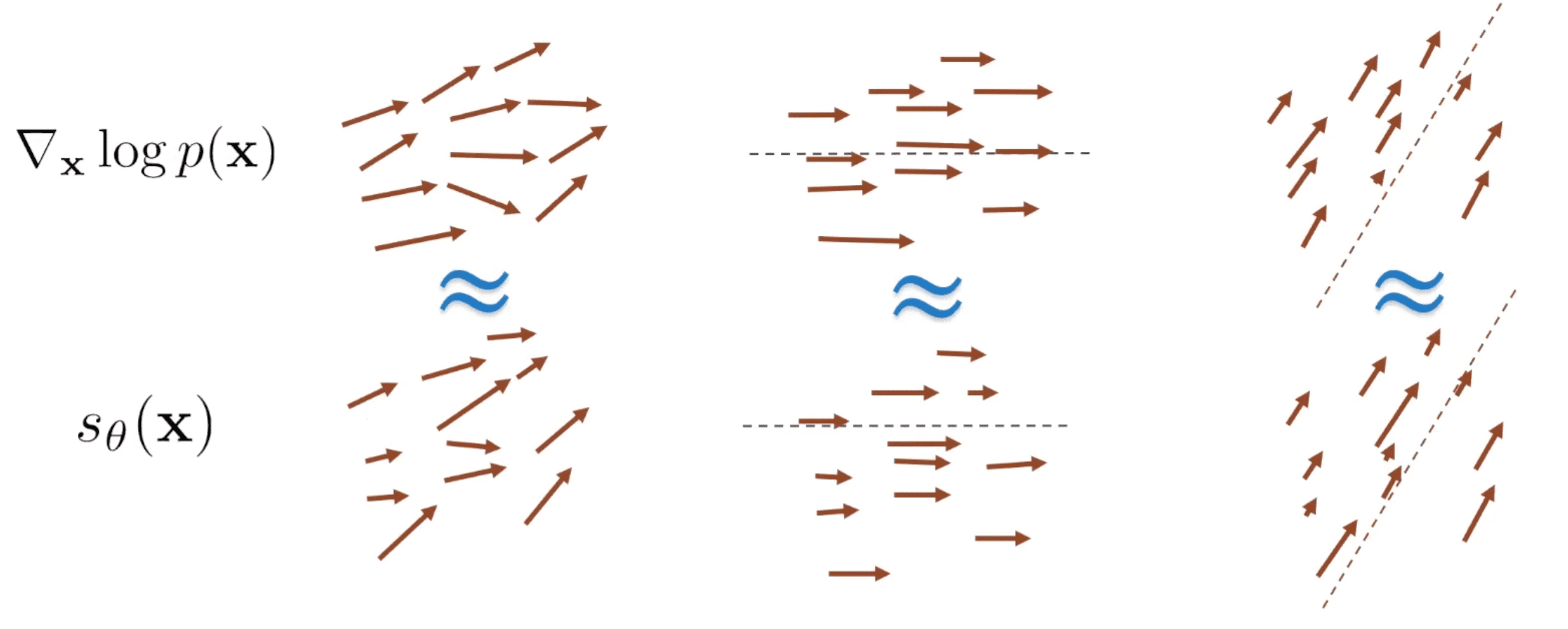
$\mathbf{Fig\ 2.}$ Sliced score matching (source: Stefano Ermon's seminar)

And with some regularity conditions, $\nabla_{\mathbf{x}} \log p_{\text{data}} (\mathbf{x})$ can be discarded by integration by parts:

$\color{red}{\mathbf{Theorem.}}$ Assume $s_{\boldsymbol{\theta}} (\mathbf{x})$, $\nabla_{\mathbf{x}} \log p_{\text{data}} (\mathbf{x})$ and $p_\mathbf{v}$ satisfy the following regularity conditions:

1. (Regularity of score functions) The model score function $s_{\boldsymbol{\theta}} (\mathbf{x})$ and data score $\nabla_{\mathbf{x}} \log p_{\text{data}} (\mathbf{x})$ are both differentiable. They additionally satisfy $\mathbb{E}_{\mathbf{x} \sim p_{\text{data}} (\mathbf{x})} [\lVert \nabla_{\mathbf{x}} \log p_{\text{data}} (\mathbf{x}) \rVert_2^2] < \infty$ and $\mathbb{E}_{\mathbf{x} \sim p_{\text{data}} (\mathbf{x})} [\lVert s_{\boldsymbol{\theta}} (\mathbf{x}) \rVert_2^2] < \infty$.
2. (Regularity of projection vectors) The projection vectors satisfy $\mathbb{E}_{\mathbf{v} \sim p_\mathbf{v}} [\lVert \mathbf{v} \rVert_2^2] < \infty$, and $\mathbb{E}_{\mathbf{v} \sim p_\mathbf{v}} [\mathbf{v}\mathbf{v}^\top] \succ 0$. (For instance, it can be multivariate standard normal, a multivariate Rademacher distribution, or a uniform distribution on the hypersphere)

Under proper boundary conditions: $\forall \boldsymbol{\theta} \in \Theta, \; \lim _{\lVert \mathbf{x} \rVert \to \infty} s_{\boldsymbol{\theta}} (\mathbf{x}) p_{\text{data}} (\mathbf{x}) = 0$, we have $$ \begin{aligned} L\left(\boldsymbol{\theta} ; p_{\mathbf{v}}\right) & \triangleq \frac{1}{2} \mathbb{E}_{\mathbf{v} \sim p_\mathbf{v}} \mathbb{E}_{\mathbf{x} \sim p_{\text{data}} (\mathbf{x})}\left[\left(\mathbf{v}^{\top} s_{\boldsymbol{\theta}} (\mathbf{x})-\mathbf{v}^{\top} \nabla_{\mathbf{x}} \log p_{\text{data}} (\mathbf{x})\right)^2\right] \\ & =\mathbb{E}_{\mathbf{v} \sim p_\mathbf{v}} \mathbb{E}_{\mathbf{x} \sim p_{\text{data}} (\mathbf{x})}\left[\mathbf{v}^{\top} \nabla_{\mathbf{x}} s_{\boldsymbol{\theta}} (\mathbf{x}) \mathbf{v}+\frac{1}{2}\left(\mathbf{v}^{\top} s_{\boldsymbol{\theta}} (\mathbf{x})\right)^2\right]+\mathrm{C}, \end{aligned} $$ where $\mathrm{C}$ is a constant w.r.t. $\boldsymbol{\theta}$.

$\mathbf{Proof.}$

Note that $L(\boldsymbol{\theta}, p_\mathbf{v})$ can be expanded to

\[\begin{aligned} & L(\boldsymbol{\theta}, p_\mathbf{v}) \\ = \; & \frac{1}{2} \mathbb{E}_{\mathbf{v} \sim p_\mathbf{v}} \mathbb{E}_{\mathbf{x} \sim p_{\text{data}} (\mathbf{x})}\left[\left(\mathbf{v}^{\top} s_{\boldsymbol{\theta}} (\mathbf{x}) -\mathbf{v}^{\top} \nabla_{\mathbf{x}} \log p_{\text{data}} (\mathbf{x})\right)^2\right] \\ \stackrel{(i)}{=} \; & \frac{1}{2} \mathbb{E}_{\mathbf{v} \sim p_\mathbf{v}} \mathbb{E}_{\mathbf{x} \sim p_{\text{data}} (\mathbf{x})}\left[\left(\mathbf{v}^{\top} s_{\boldsymbol{\theta}} (\mathbf{x}) \right)^2+\left(\mathbf{v}^{\top} \nabla_{\mathbf{x}} \log p_{\text{data}} (\mathbf{x})\right)^2-2\left(\mathbf{v}^{\top} s_{\boldsymbol{\theta}} (\mathbf{x}) \right)\left(\mathbf{v}^{\top} \nabla_{\mathbf{x}} \log p_{\text{data}} (\mathbf{x})\right)\right] \\ = \; &\mathbb{E}_{\mathbf{v} \sim p_\mathbf{v}} \mathbb{E}_{\mathbf{x} \sim p_{\text{data}} (\mathbf{x})}\left[-\left(\mathbf{v}^{\top} s_{\boldsymbol{\theta}} (\mathbf{x}) \right)\left(\mathbf{v}^{\top} \nabla_{\mathbf{x}} \log p_{\text{data}} (\mathbf{x})\right)+\frac{1}{2}\left(\mathbf{v}^{\top} x \right)^2\right]+\mathrm{C}, \end{aligned}\]

where $(i)$ is due to the assumptions of bounded expectations. Now it suffices to show that

\[\begin{aligned} - \mathbb{E}_{\mathbf{v} \sim p_\mathbf{v}} \mathbb{E}_{\mathbf{x} \sim p_{\text{data}} (\mathbf{x})} [(\mathbf{v}^\top s_{\boldsymbol{\theta}} (\mathbf{x}))(\mathbf{v}^\top \nabla_{\mathbf{x}} \log p_{\text{data}} (\mathbf{x}))] = \mathbb{E}_{\mathbf{v} \sim p_\mathbf{v}} \mathbb{E}_{\mathbf{x} \sim p_{\text{data}} (\mathbf{x})} [\mathbf{v}^\top \nabla_{\mathbf{x}} s_{\boldsymbol{\theta}} (\mathbf{x}) \mathbf{v}]. \end{aligned}\]

First, observe that

\[\begin{aligned} & - \mathbb{E}_{\mathbf{v} \sim p_\mathbf{v}} \mathbb{E}_{\mathbf{x} \sim p_{\text{data}} (\mathbf{x})} [(\mathbf{v}^\top s_{\boldsymbol{\theta}} (\mathbf{x}))(\mathbf{v}^\top \nabla_{\mathbf{x}} \log p_{\text{data}} (\mathbf{x}))] \\ = \; &-\mathbb{E}_{\mathbf{v} \sim p_\mathbf{v}} \int p_{\text{data}} (\mathbf{x})\left(\mathbf{v}^{\top} s_{\boldsymbol{\theta}} (\mathbf{x})\right)\left(\mathbf{v}^{\top} \mathbf{s}_d(\mathbf{x} ; \boldsymbol{\theta})\right) \mathrm{d} \mathbf{x} \\ = \; &-\mathbb{E}_{\mathbf{v} \sim p_\mathbf{v}} \int p_{\text{data}} (\mathbf{x})\left(\mathbf{v}^{\top} s_{\boldsymbol{\theta}} (\mathbf{x})\right)\left(\mathbf{v}^{\top} \nabla_{\mathbf{x}} \log p_{\text{data}} (\mathbf{x})\right) \mathrm{d} \mathbf{x} \\ = \; &-\mathbb{E}_{\mathbf{v} \sim p_\mathbf{v}} \int\left(\mathbf{v}^{\top} s_{\boldsymbol{\theta}} (\mathbf{x})\right)\left(\mathbf{v}^{\top} \nabla_{\mathbf{x}} p_{\text{data}} (\mathbf{x})\right) \mathrm{d} \mathbf{x} \\ = \; &-\mathbb{E}_{\mathbf{v} \sim p_\mathbf{v}} \sum_{i=1}^D \int\left(\mathbf{v}^{\top} s_{\boldsymbol{\theta}} (\mathbf{x})\right) v_i \frac{\partial p_{\text{data}} (\mathbf{x})}{\partial x_i} \mathrm{~d} \mathbf{x}, \end{aligned}\]

where we assume that $\mathbf{x} \in \mathbb{R}^{\mathrm{D}}$. By applying multivariate integration by parts, we obtain

\[\begin{aligned} &\left|\mathbb{E}_{\mathbf{v} \sim p_\mathbf{v}} \sum_{i=1}^D \int\left(\mathbf{v}^{\top} s_{\boldsymbol{\theta}} (\mathbf{x})\right) v_i \frac{\partial p_{\text{data}}(\mathbf{x})}{\partial x_i} \mathrm{~d} \mathbf{x}+\mathbb{E}_{\mathbf{v} \sim p_\mathbf{v}} \sum_{i=1}^D \int v_i p_{\text{data}}(\mathbf{x}) \mathbf{v}^{\top} \frac{\partial s_{\boldsymbol{\theta}} (\mathbf{x})}{\partial x_i} \mathrm{~d} \mathbf{x}\right| \\ &=\left|\mathbb{E}_{\mathbf{v} \sim p_\mathbf{v}}\left[\sum_{i=1}^D \lim _{x_i \rightarrow \infty}\left(\mathbf{v}^{\top} s_{\boldsymbol{\theta}} (\mathbf{x})\right) v_i p_{\text{data}}(\mathbf{x})-\sum_{i=1}^D \lim _{x_i \rightarrow-\infty}\left(\mathbf{v}^{\top} s_{\boldsymbol{\theta}} (\mathbf{x})\right) v_i p_{\text{data}}(\mathbf{x})\right]\right| \\ & \leq \sum_{i=1}^D \lim _{x_i \rightarrow \infty} \sum_{j=1}^D \mathbb{E}_{\mathbf{v} \sim p_\mathbf{v}}\left|v_i v_j\right|\left|s_{\boldsymbol{\theta}} (\mathbf{x})_j p_{\text{data}}(\mathbf{x})\right|+\sum_{i=1}^D \lim _{x_i \rightarrow-\infty} \sum_{j=1}^D \mathbb{E}_{\mathbf{v} \sim p_\mathbf{v}}\left|v_i v_j\right|\left|s_{\boldsymbol{\theta}} (\mathbf{x})_j p_{\text{data}}(\mathbf{x})\right| \\ & \stackrel{(i)}{\leq} \sum_{i=1}^D \lim _{x_i \rightarrow \infty} \sum_{j=1}^D \sqrt{\mathbb{E}_{\mathbf{v} \sim p_\mathbf{v}} v_i^2 \mathbb{E}_{\mathbf{v} \sim p_\mathbf{v}} v_j^2}\left|s_{\boldsymbol{\theta}} (\mathbf{x})_j p_{\text{data}}(\mathbf{x})\right|+\sum_{i=1}^D \lim _{x_i \rightarrow-\infty} \sum_{j=1}^D \sqrt{\mathbb{E}_{\mathbf{v} \sim p_\mathbf{v}} v_i^2 \mathbb{E}_{\mathbf{v} \sim p_\mathbf{v}} v_j^2}\left|s_{\boldsymbol{\theta}} (\mathbf{x})_j p_{\text{data}}(\mathbf{x})\right| \\ & \stackrel{(i i)}{=} 0 \end{aligned}\]

where \(s_{\boldsymbol{\theta}} (\mathbf{x})_j\) denotes the \(j\)-th component of \(s_{\boldsymbol{\theta}} (\mathbf{x})\). And $(i)$ is due to Cauchy-Schwartz inequality and $(ii)$ is from the assumption that \(\mathbb{E}_{\mathbf{v} \sim p_{\mathbf{v}}} [\lVert \mathbf{v} \rVert_2^2] < \infty\) and \(s_{\boldsymbol{\theta}} (\mathbf{x})\) vanishes at infinity.

By combining these results, we have

\[\begin{aligned} & - \mathbb{E}_{\mathbf{v} \sim p_\mathbf{v}} \sum_{i=1}^D \int (\mathbf{v}^\top s_{\boldsymbol{\theta}} (\mathbf{x})) v_i \frac{\partial p_{\text{data}} (\mathbf{x})}{\partial x_i} d\mathbf{x} \\ = \; & \mathbb{E}_{\mathbf{v} \sim p_\mathbf{v}} \sum_{i=1}^\mathrm{D} \int v_i p_{\text{data}} (\mathbf{x}) \mathbf{v}^\top \frac{\partial s_{\boldsymbol{\theta}} (\mathbf{x})}{\partial x_i} d\mathbf{x} \\ = \; & \mathbb{E}_{\mathbf{v} \sim p_\mathbf{v}} \int p_{\text{data}} \mathbf{v}^\top \nabla_{\mathbf{x}} s_{\boldsymbol{\theta}} (\mathbf{x}) \mathbf{v} d \mathbf{x}, \end{aligned}\]

which shows the theorem.

\[\tag*{$\blacksquare$}\]

II. Langevin Dynamics: Sampling from the score

Langevin Dynamics allows us to produce samples from $p (\mathbf{x})$ using only the score function $\nabla_{\mathbf{x}} \text{ log } p(\mathbf{x})$. Given a fixed step size $\varepsilon > 0$, and an initial value $\tilde{\mathbf{x}}_0 \sim \pi (\mathbf{x})$ from a prior distribution $\pi$, the Langevin method recursively computes

\[\begin{aligned} \tilde{\mathbf{x}}_t = \tilde{\mathbf{x}}_{t - 1} + \frac{\varepsilon}{2} \nabla_{\mathbf{x}} \text{ log } p(\tilde{\mathbf{x}}_{t-1}) + \sqrt{\varepsilon} \mathbf{z}_{t} \quad \text{ where } \quad \mathbf{z}_t \sim \mathcal{N}(\mathbf{0}, \mathbf{I}) \end{aligned}\]

And the distribution of \(\tilde{\mathbf{x}}_t\) converges to $p(\mathbf{x})$ when $\varepsilon \to 0$ and $t \to \infty$ under some regularity conditions. For further insights on this matter, I highly recommend reading Paweł A. Pierzchlewicz’s excellently crafted post. Below, I briefly summarized his post.

$\mathbf{Summary.}$

(Reference: [5])

In the realm of physics, Langevin dynamics serves as an approach to mathematically model the dynamics of molecular systems. Originating from the mind of the French physicist Paul Langevin, the foundational Langevin equation describes Brownian motion, the random movement of a particle within a fluid due to collisions with the molecules of the fluid:

\[\begin{aligned} m \frac{d \mathbf{v}}{dt} = - \lambda \mathbf{v} + \boldsymbol{\eta} (t) \end{aligned}\]

where $\mathbf{v}$ stands for the velocity of the particle, $\lambda$ is its damping coefficient, $m$ is its mass, and $\boldsymbol{\eta} (t) \sim \mathcal{N} (0, 2 \sigma^2)$ is a Gaussian noise at time $t$. As force is the negative gradient of potential energy $V(\mathbf{x})$, we have

\[\begin{aligned} \nabla V(\mathbf{x}) = \lambda \mathbf{v} - \boldsymbol{\eta} (t) = \lambda \frac{d\mathbf{x}}{dt} - \boldsymbol{\eta} (t) \end{aligned}\]

Our next step is to rewrite the equation in the form of stochastic differential eqaution. To this end, note that the definition of Wiener process:

1. $W$ has Gaussian increments: The change $\Delta W$ during a small period of time $\Delta t$ is $\Delta W = \varepsilon \sqrt{\Delta t}$, where $\varepsilon \sim \mathcal{N}(0, 1)$.
2. $W$ has independent increments

Thus, from $dW = \varepsilon dt$ and $\boldsymbol{\eta (t)} = \sqrt{2} \sigma \varepsilon$, we can rewrite it in stochastic differential eqaution:

\[\begin{aligned} d \mathbf{x} = - \nabla V(\mathbf{x}) dt + \sqrt{2} \sigma dW \end{aligned}\]

To describe the time evolution of the probability density function $p(\mathbf{x}, t)$ of the velocity of a particle (under the influence of drag forces and random forces, as in Brownian motion), we have Fokker-Planck equation, which is defined for a typical SDE

\[\begin{aligned} dx = \mu(x, t) dt + \sigma(x, t) dW \end{aligned}\]

with drift $\mu (x, t)$ and diffusion coefficient $D(x, t) = \sigma (x, t)^2 / 2$. For such SDE the Fokker-Planck equation for the probability density $p (x, t)$ is

\[\begin{aligned} \frac {\partial }{\partial t} p(x, t)=- \frac {\partial }{\partial x}\left[\mu (x,t)p(x,t)\right]+{\frac {\partial ^{2}}{\partial x^{2}}}\left[D(x,t)p(x,t)\right]. \end{aligned}\]

Thus for our SDE from Lagevin equation we have

\[\begin{aligned} \frac {\partial }{\partial t} p(\mathbf{x}, t)= \frac {\partial }{\partial \mathbf{x}}\left[ \nabla V(\mathbf{x}) p(\mathbf{x},t)+ \frac {\partial}{\partial \mathbf{x}}\left(\sigma^2 p(\mathbf{x},t) \right)\right]. \end{aligned}\]

We are interested in the steady state (i.e. $\partial p(\mathbf{x}, t) / \partial t = 0$) distribution $p(\mathbf{x})$. That is, for any $\mathbf{x}$,

\[\begin{aligned} \frac {\partial }{\partial t} p(\mathbf{x})= \frac {\partial }{\partial \mathbf{x}} \left [ \nabla V(\mathbf{x}) p(\mathbf{x}) +{\frac {\partial}{\partial \mathbf{x}}}\left(\sigma^2 p(\mathbf{x})\right) \right] = 0. \end{aligned}\]

In other words,

\[\begin{aligned} \frac{\partial}{\partial \mathbf{x}} p(\mathbf{x}) = - \frac{\nabla V(\mathbf{x})}{\sigma^2} p(\mathbf{x}) \end{aligned}\]

which implies

\[\begin{aligned} p(\mathbf{x}) \propto \text{ exp } \left(- \frac{V(\mathbf{x})}{\sigma^2} \right) \end{aligned}\]

Thus, for $\sigma = 1$ we finalize that we have to set the potential energy to be $\text{log } p(x)$ to sample from the distribution $p(x)$. Now let’s turn back to our sampling. We rewrite the stochastic differential equation in terms of the target distribution $p_{\text{data}} (\mathbf{x})$ with $\sigma = 1$:

\[\begin{aligned} d \mathbf{x} = \nabla_{\mathbf{x}} \text{ log } p_{\text{data}} (\mathbf{x}) dt + \sqrt{2} dW \end{aligned}\]

One of the simplest way to solve the SDE numerically is Euler-Maruyama method, which recursively computes

\[\begin{aligned} \mathbf{x}_{n + 1} = \mathbf{x}_n + \nabla_{\mathbf{x}} \text{ log } p_{\text{data}} (\mathbf{x}) \varepsilon + \sqrt{2 \varepsilon} \mathbf{z}_n \quad \text{ where } \quad \mathbf{z}_n \sim \mathcal{N}(\mathbf{0}, \mathbf{I}) \end{aligned}\]

where $\varepsilon$ is the time step. And it is known that Euler-Maruyama converges as $n \to \infty$ and $\varepsilon \to 0$ under some regularity conditions. Equivalently, by substituting $\varepsilon$ by $\varepsilon / 2$ we may obtain

\[\begin{aligned} \mathbf{x}_{n + 1} = \mathbf{x}_n + \nabla_{\mathbf{x}} \text{ log } p_{\text{data}} (\mathbf{x}) \frac{\varepsilon}{2} + \sqrt{\varepsilon} \mathbf{z}_n \quad \text{ where } \quad \mathbf{z}_n \sim \mathcal{N}(\mathbf{0}, \mathbf{I}) \end{aligned}\]

which we desired.

\[\tag*{$\blacksquare$}\]

Consequently, so as to sample from unknown $p_{\text{data}} (\mathbf{x})$, we first train score network $s_{\boldsymbol{\theta}} (\mathbf{x}) \approx \nabla_{\mathbf{x}} \text{ log } p_{\text{data}} (\mathbf{x})$ and then approximately obtain samples from Langevin dynamics using $s_{\boldsymbol{\theta}} (\mathbf{x})$ instead of $p_{\text{data}} (\mathbf{x})$.

Challenges

There are two major challenges that hinder the convergence and performance of score-based generative models.

I. Manifold hypotheses

The manifold hypothesis suggests that numerous high-dimensional datasets encountered in the real world reside along low-dimensional latent manifolds within that high-dimensional space (the ambient space). Consequently, datasets that initially require many variables to represent, can be reduced into comparatively small number of variables, thereby supporting the effectiveness of machine learning algorithms describing high-dimensional datasets within few features.

And in accordance with the manifold hypothesis, score-based generative models encounter two primary obstacles:

1. The score $\nabla_{\mathbf{x}} \text{ log } p_{\text{data}} (\mathbf{x})$ is approximated in the ambient space, thereby being collapsed if $\mathbf{x}$ is confined to low-dimensional manifold.
2. The regularity assumptions that ensures the consistency of score estimator are collapsed if the support of the data distribution is not the whole space.

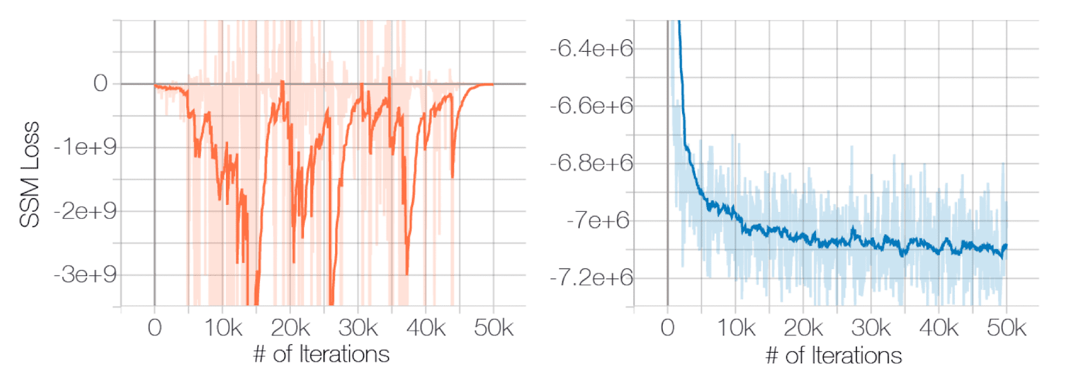
And the negative effect of described problems is posited by the experimental results conducted by Song and Ermon et al. NeurIPS 2019. The following figure shows the failure of convergence of score matching with ResNet on CIFAR-10:

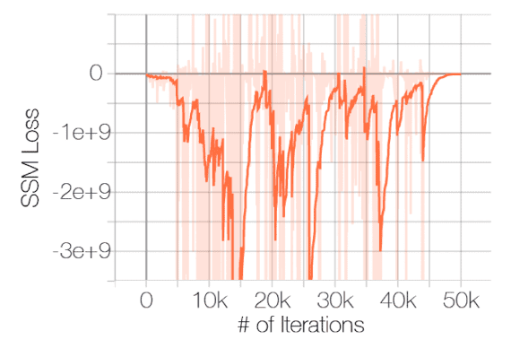
$\mathbf{Fig\ 3.}$ Sliced score matching loss w.r.t iterations (source: [2])

II. Low data density regions

The low density regions hamper both score estimation and sampling with Langevin dynamics. Since score is estimated based on the i.i.d data samples \(\{ \mathbf{x}_n \}_{n=1}^N \sim p_{\text{data}} (\mathbf{x})\), the algorithm may not have enough evidence to estimate score functions accurately in low data density regions.

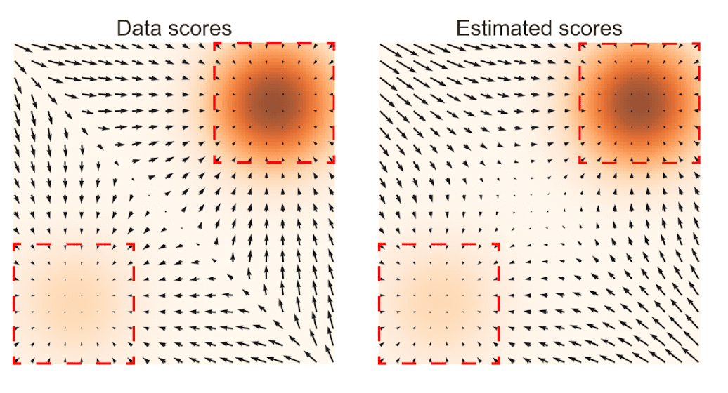
$\mathbf{Fig\ 4.}$ Left: $\nabla_{\mathbf{x}} \text{ log } p_{\text{data}} (\mathbf{x})$ Right: $\mathbf{s}_{\boldsymbol{\theta}} (\mathbf{x})$ (source: [2])

Furthermore, when more than two modes of the data distribution are divided by regions of low density such as $\mathbf{Fig\ 4.}$, Langevin dynamics may struggle to accurately capture the relative weights of these two modes within the reasonable number of time steps. Formally, consider the mixture data distribution

\[\begin{aligned} p_{\text{data}} (\mathbf{x}) = \pi p_1 (\mathbf{x}) + (1 - \pi) p_2 (\mathbf{x}) \end{aligned}\]

where the weight $\pi \in (0, 1)$, $p_1$ and $p_2$ are normalized distributions with disjoint supports $S_1$ and $S_2$. Then, for both supports $S_1$ and $S_2$, the score will be independent of $\pi$:

\[\begin{aligned} \nabla_{\mathbf{x}} \text{ log } p_{\text{data}} (\mathbf{x}) = \begin{cases} \nabla_{\mathbf{x}} (\pi + \text{ log } p_1 (\mathbf{x})) = \nabla_{\mathbf{x}} \text{ log } p_1 (\mathbf{x}) & \quad \mathbf{x} \in S_1 \\ \nabla_{\mathbf{x}} (\pi + \text{ log } p_2 (\mathbf{x})) = \nabla_{\mathbf{x}} \text{ log } p_2 (\mathbf{x}) & \quad \mathbf{x} \in S_2 \end{cases} \end{aligned}\]

Since Langevin dynamics obtains samples from $p_{\text{data}} (\mathbf{x})$ only with samples from $\nabla_{\mathbf{x}} \text{ log } p_{\text{data}} (\mathbf{x})$, the samples will not depend on $\pi$. In this regime, it may require extremely small step size and large number of time steps to correctly sample from the mixed distribution.

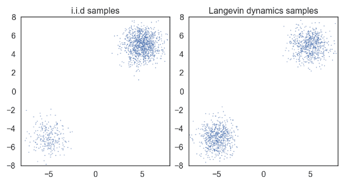
$\mathbf{Fig\ 5.}$ Samples obtained from a mixture of Gaussian with different sampling methods
(a) exact sampling (b) Langevin dynamics with the exact scores. (source: [2])

Noise Conditional Score Networks (NCSN)

Song and Ermon et al., NeurIPS 2019 found that the perturbation of data by random Gaussian noise makes the data distribution amenable to score-based generative modeling as it mitigates the issues we’ve discussed as follows:

• since the support of the Gaussian distribution is the whole space, the perturbed data will not be confined to a low dimensional manifold and makes score matching well-defined
• large Gaussian noise fills the low density regions in the original data distribution

On top of this intuitions, noise conditional score networks (NCSN) improve the score-based generative modeling framework by

1. perturbing the data using various levels of noise $\{ \sigma_i \}_{i=1}^L$
2. estimating scores corresponding to all noise levels with a single noise conditional score network $\mathbf{s}_{\boldsymbol{\theta}} (\mathbf{x}, \sigma)$
3. sampling with annealed Lagevin dynamics; initially use scores corresponding to large noise levels and gradually anneal down the noise level.

Note that the design of neural network architectures contributes to generating the high quality samples in a large amount. Since the output of NCSN has the same shape as the input image $\mathbf{x}$, the authors harnessed the successful model architectures for image dense prediction tasks such as U-Net.

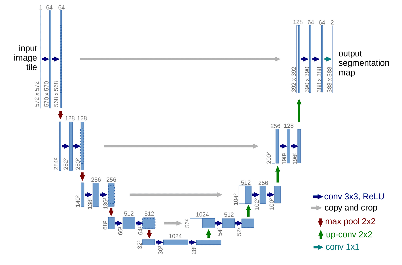
$\mathbf{Fig\ 6.}$ U-Net Architecture. Originally proposed for biomedical image segmentation (source: Olaf et al. 2015)

Training: Denoising score matching

The training of NCSN amounts to the denoising score matching, with the only difference that we regulate the levels of perturbation. Let \(\{ \sigma_n \}_{n=1}^L\) be a positive geometric sequence that satisfies $\frac{\sigma_1}{\sigma_2} = \cdots = \frac{\sigma_{L-1}}{\sigma_{L}} > 1$. To obviate the challenges $\sigma_1$ should be large enough, but $\sigma_L$ should be smalle enough to minimize the effect on the data. Denote the perturbed data distribution with noise level $\sigma$ as

\[\begin{aligned} q_{\sigma} (\widetilde{\mathbf{x}}) = \int q_{\sigma} (\widetilde{\mathbf{x}} \mid \mathbf{x}) p_{\text{data}} (\mathbf{x}) \; d\mathbf{x} = \int p_{\text{data}} (\mathbf{x}) \mathcal{N} (\widetilde{\mathbf{x}} \mid \mathbf{x}, \sigma^2 \mathbf{I}) \; d\mathbf{x} \end{aligned}\]

We choose the noise distribution $q_{\sigma} (\widetilde{\mathbf{x}} \mid \mathbf{x}) = \mathcal{N} (\widetilde{\mathbf{x}} \mid \mathbf{x}, \sigma^2 \mathbf{I})$. Hence the denoising score matching objective is

\[\begin{aligned} \ell(\boldsymbol{\theta} ; \sigma) = \frac{1}{2} \mathbb{E}_{p_{\text {data }}(\mathbf{x})} \mathbb{E}_{\tilde{\mathbf{x}} \sim \mathcal{N}\left(\mathbf{x}, \sigma^2 I\right)}\left[\left\|\mathbf{s}_{\boldsymbol{\theta}}(\tilde{\mathbf{x}}, \sigma)+\frac{\tilde{\mathbf{x}}-\mathbf{x}}{\sigma^2}\right\|_2^2\right] \end{aligned}\]

and the unified objective for all \(\sigma \in \{ \sigma_n \}_{n=1}^L\) is

\[\begin{aligned} \mathcal{L} (\boldsymbol{\theta} ; \{ \sigma_n \}_{n=1}^L) = \frac{1}{L} \sum_{n=1}^L \lambda (\sigma_n) \ell (\boldsymbol{\theta} ; \sigma_n) \end{aligned}\]

where $\lambda(\sigma_n) > 0$ is a coefficient function.

choice of $\lambda$

Emprically, the authors observe that when the score networks are trained to optimality, \(\lVert \mathbf{s}_{\boldsymbol{\theta}} (\mathbf{x}, \sigma) \rVert_2 \propto 1 / \sigma\). And this gives us the inspiration to choose $\lambda (\sigma) = 1 / \sigma^2$; since we will have $\lambda(\sigma) \ell (\boldsymbol{\theta} ; \sigma)$ indepedent of $\sigma$ as $\frac{\widetilde{\mathbf{x}} - \mathbf{x}}{\sigma} = \mathcal{N} (0, \sigma \mathbf{I})$.

$\mathbf{Fig\ 7.}$ Perturbing the data (right) well-defines the score estimation (source: [2])

Inference: Annealed Langevin dynamics

To sample from noise conditional score network, we need a slighted modified version of Langevin dynamics, so-called annealed Langevin dynamics inspired by simulated annealing and annealed importance sampling:

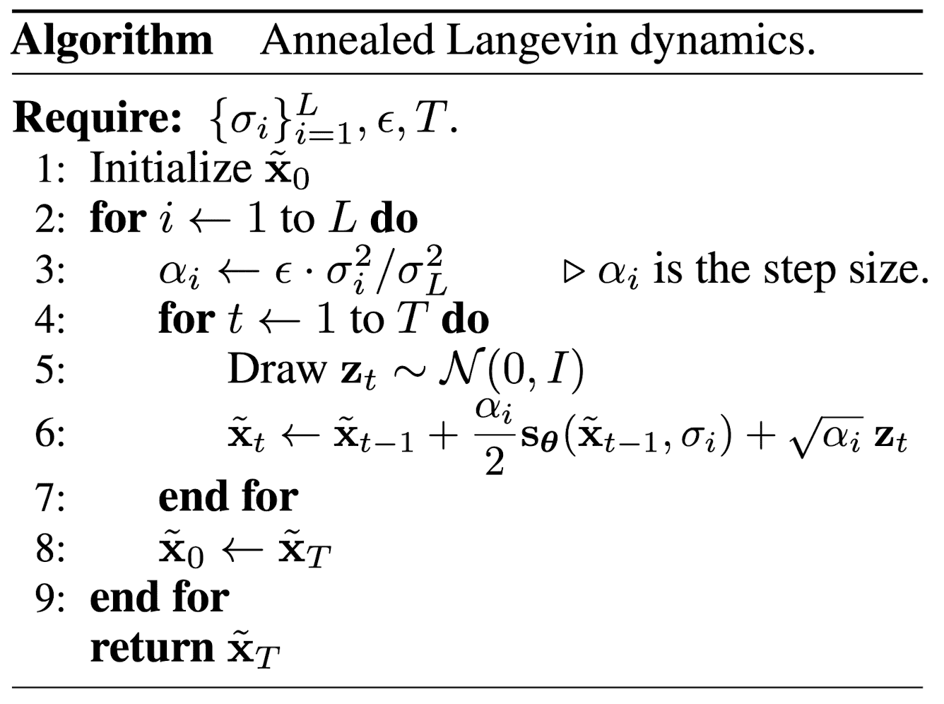
$\mathbf{Fig\ 8.}$ Annealed Langevin Dynamics (source: [2])

Heuristically speaking, the simulated annealing is an algorithm that maintains a current solution and iteratively explores neighboring solutions. At each iteration, it probabilistically accepts worse solutions with the hope of escaping local optima and finding a global optimum. The probability of accepting a worse solution decreases over time based on some annealing schedule (may be specified by the user, but must end with zero), resembling the cooling process in metallurgy.

$\mathbf{Fig\ 9.}$ Simulated annealing for optimization (source: wikimedia)

Built upon this inspiration, we run Langevin dynamics inductively to sample $\widetilde{\mathbf{x}}$ from the distribution $q_{\sigma_n} (\mathbf{x})$ corresponding to noise level $\sigma_n$, and starting from the final samples $\widetilde{\mathbf{x}}$ of $q_{\sigma_n} (\mathbf{x})$ as the initial samples and tuning down the step size $\alpha_n$ gradually, obtain a sample from the distribution $q_{\sigma_{n + 1}} (\mathbf{x})$.

Since the supports of perturbed distributions span the whole space by Gaussian noise and their scores are well-defined in terms of regularity conditions, it is possible to circumvent the obstacles from the manifold hypothesis. Also, if $\sigma_1$ is sufficiently large, the low density regions of $q_{\sigma_1}$ will be filled and it makes score estimation more accurate and also modes less isolated, thereby improving the mixing speed of Langevin dynamics more faster. And the following empirical result justifies the hypothesis:

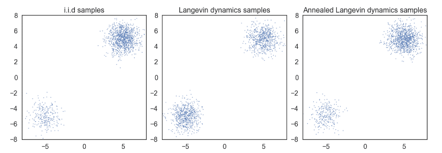
$\mathbf{Fig\ 10.}$ Annealed Langevin dynamics improves the mixing (source: [2])

As score estimation and Langevin dynamics perform better in high density regions, samples from $q_{\sigma_1}$ will serve as good initial samples for Langevin dynamics of $q_{\sigma_2}$. Inductively, $q_{\sigma_{n-1}}$ provides good initial samples for $q_{\sigma_n}$, and finally we obtain samples of good quality from $q_{\sigma_L}$.

choice of $\alpha_n$

The authors choice is $\alpha_n \propto \sigma_n^2$. The inspiration comes from the intuitive desire to fix the signal-to-noise ratio $\frac{\alpha_n \mathbf{s}_{\boldsymbol{\theta}} (\mathbf{x}, \sigma_n)}{2 \sqrt{\alpha_n} \mathbf{z}}$ in Langevin dynamics, with respect to the noise level.

Note that

\[\begin{aligned} \mathbb{E}\left[\left\|\frac{\alpha_n \mathbf{s}_{\boldsymbol{\theta}}\left(\mathbf{x}, \sigma_n \right)}{2 \sqrt{\alpha_n } \mathbf{z}}\right\|_2^2\right] \approx \mathbb{E}\left[\frac{\alpha_n \left\|\mathbf{s}_{\boldsymbol{\theta}}\left(\mathbf{x}, \sigma_n \right)\right\|_2^2}{4}\right] \propto \frac{1}{4} \mathbb{E}\left[\left\|\sqrt{\alpha_n} \mathbf{s}_{\boldsymbol{\theta}}\left(\mathbf{x}, \sigma_n \right)\right\|_2^2\right] \end{aligned}\]

From the empirical observation $|| \mathbf{s}_{\boldsymbol{\theta}}\left(\mathbf{x}, \sigma_n\right) ||_2 \propto 1/\sigma_n$, it is desirable to set $\alpha_n \propto \sigma_n^2$.

Reference

[1] Sohl-Dickstein, Jascha, et al. “Deep unsupervised learning using nonequilibrium thermodynamics.” ICML 2015..
[2] Song and Ermon, “Generative Modeling by Estimating Gradients of the Data Distribution”, NeurIPS 2019.
[3] Hyvärinen, Aapo, and Peter Dayan. “Estimation of non-normalized statistical models by score matching.” JMLR 2005.
[4] Vincent, Pascal. “A connection between score matching and denoising autoencoders.” Neural computation 23.7 (2011): 1661-1674.
[5] Pierzchlewicz, Paweł A. (Jul 2022). Langevin Monte Carlo: Sampling using Langevin Dynamics. Perceptron.blog.
[6] Song, Yang, et al., Sliced Score Matching: A Scalable Approach to Density and Score Estimation, Uncertainty in Artificial Intelligence. PMLR, 2020.