[Generative Model] Diffusion Probabilistic Models

This post is about the fundamentals of diffusion model.

Diffusion Probabilistic Models (DPM)

Diffusion probabilistic model, proposed by Sohl-Dickstein et al., ICML 2015, is a foundation paper of Denoising Diffusion Probabilistic Models (DDPMs).

Introduction

Probabilistic models usually suffer from a trade-off between tractability and flexibility.

• Tractability
  • (+) learning, sampling, inference, etc. can be analytically evaluated
  • (-) unable to aptly express complex distributions
• Flexibility
  • (+) can be fitted to structure of arbitrary data
  • (-) generally include intractable operations

The authors proposed a novel probabilistic models, inspired by non-equilibrium statistical physics, with desirable properties:

1. extreme flexibility
2. exact sampling
3. easy multiplication with other distributions and normalization, e.g. to compute posterior
4. cheaply computable log likelihood and probability

Algorithm

The entire pipeline of algorithm is as follows.

1. Forward Process converts complex data distribution into simple tractable distribution
2. Reverse Process learn (finite-time) reverse process that is a reversal of forward trajectory

And the reverse process defines our generative model distribution. Before we start, let’s first define notations:

• $q( \mathbf{x}^{(0)} )$: data distribution
• $q ( \mathbf{x}^{(t)} \mid \mathbf{x}^{(t-1)} )$: forward process
• $\pi ( \mathbf{y} )$: tractable distribution
  • $T$ stands for step numbers of diffusion
  • We define $p ( \mathbf{x}^{(T)}) = \pi ( \mathbf{x}^{(T)})$
• $p ( \mathbf{x}^{(t - 1)} \mid \mathbf{x}^{(t)})$: reverse process

Hence the objective of training models is ..

Forward process

The data distribution $q( \mathbf{x}^{(0)} )$ is gradually converted into a tractable distribution $\pi (\mathbf{y})$ by repeated application of $q ( \mathbf{x}^{(t)} \mid \mathbf{x}^{(t-1)})$. Starting at the data distribution and performing $T$ steps of diffusion, we have

\[\begin{aligned} q \left( \mathbf{x}^{(0)}, \cdots \mathbf{x}^{(T)} \right) = q \left( \mathbf{x}^{(0 \dots T)} \right) = q \left( \mathbf{x}^{(0)} \right) \prod_{t=1}^T q \left( \mathbf{x}^{(t)} \mid \mathbf{x}^{(t-1)} \right) \end{aligned}\]

In the paper, the authors set $q \left( \mathbf{x}^{(t)} \mid \mathbf{x}^{(t-1)} \right)$ to either Gaussian diffusion into a Gaussian distribution with identity-covariance, or binomial diffusion into an independent binomial distribution.

\[\begin{aligned} q \left( \mathbf{x}^{(t)} \mid \mathbf{x}^{(t-1)} \right) = \begin{cases} \mathcal{N} (\mathbf{x}^{(t)} ; \mathbf{x}^{(t-1)} \sqrt{1 - \beta_t}, \mathbb{I} \beta_t) & \quad \text{Gaussian} \\ \mathcal{B} (\mathbf{x}^{(t)} ; \mathbf{x}^{(t-1)} (1 - \beta_t) + 0.5 \beta_t) & \quad \text{Binomial} \end{cases} \end{aligned}\]

Reverse process

In reverse,

\[\begin{aligned} p \left(\mathbf{x}^{(T)} \right) & := \pi \left(\mathbf{x}^{(T)} \right) \\ p \left( \mathbf{x}^{(0)}, \cdots \mathbf{x}^{(T)} \right) & = p \left( \mathbf{x}^{(0 \dots T)} \right) = p \left( \mathbf{x}^{(T)} \right) \prod_{t=1}^T p \left( \mathbf{x}^{(t-1)} \mid \mathbf{x}^{(t)} \right) \end{aligned}\]

In 1949, W. Feller showed that, for gaussian (and binomial) distributions, the diffusion process’s reversal has the same functional form as the forward process. If $\beta_t$ in Gaussian (respectively, binomial) \(q( \mathbf{x}^{(t)} \mid \mathbf{x}^{(t-1)})\) is small, the reverse \(q( \mathbf{x}^{(t-1)} \mid \mathbf{x}^{(t)})\) will also be a Gaussian (respectively, binomial).

Therefore we let the neural network to estimate the parameters of distributions:

\[\begin{aligned} p \left( \mathbf{x}^{(t-1)} \mid \mathbf{x}^{(t)} \right) = \begin{cases} \mathcal{N} (\mathbf{x}^{(t-1)} ; \mathbf{f}_{\mu} (\mathbf{x}^{(t)}, t), \mathbf{f}_{\Sigma} (\mathbf{x}^{(t)}, t) ) & \quad \text{Gaussian} \\ \mathcal{B} (\mathbf{x}^{(t-1)} ; \mathbf{f}_b ( \mathbf{x}^{(t)}, t )) & \quad \text{Binomial} \end{cases} \end{aligned}\]

Model Probability

Before we delve into training, we need to compute the probability the generative model assgins to the data.

\[\begin{aligned} p (\mathbf{x}^{(0)}) = \int dx^{(1 \cdots T)} p(x^{(0 \cdots T)}) \end{aligned}\]

To deal with intractability, we modify the integral:

\[\begin{aligned} p(x^{(0)}) &= \int dx^{(1 \cdots T)} p(x^{(0 \cdots T)}) \frac{q(x^{(1 \cdots T)} \mid x^{(0)})}{q(x^{(1 \cdots T)} \mid x^{(0)})} \\ &= \int dx^{(1 \cdots T)} q(x^{(1 \cdots T)} \mid x^{(0)}) \frac{p(x^{(0 \cdots T)})}{q(x^{(1 \cdots T)} \mid x^{(0)})} \\ &= \int dx^{(1 \cdots T)} q(x^{(1 \cdots T)} \mid x^{(0)}) p(x^{(T)}) \prod_{t=1}^T \frac{p(x^{(t-1)} \mid x^{(t)})}{q(x^{(t)} \mid x^{(t-1)})} \end{aligned}\]

Recall that for infinitesimal $\beta$ the forward and reverse distribution over trajectories can be made identical. Therefore it is computable with only a single sample from \(q(x^{(1 \cdots T)} \mid x^{(0)})\).

Training

Training aims to maximize the log likelihood $L$ of model:

\[\begin{aligned} L = \mathbb{E}_{\mathbf{x}^{(0)} \sim q (\cdot)} \left[ \text{ log } p (\mathbf{x}^{(0)}) \right] & = \int dx^{(0)} q(x^{(0)}) \log p(x^{(0)}) \\ & = \int dx^{(0)} q(x^{(0)}) \log \left[ \int dx^{(1 \cdots T)} q(x^{(1 \cdots T)} \mid x^{(0)}) p(x^{(T)}) \prod_{t=1}^T \frac{p(x^{(t-1)} \mid x^{(t)})}{q(x^{(t)} \mid x^{(t-1)})} \right] \end{aligned}\]

which has a lower bound $K$ by Jensen’s inequality:

\[\begin{aligned} L & \geq \int dx^{(0 \cdots T)} q(x^{(0 \cdots T)}) \log \left[ p(x^{(T)}) \prod_{t=1}^T \frac{p(x^{(t-1)} \mid x^{(t)})}{q(x^{(t)} \mid x^{(t-1)})} \right] = K \end{aligned}\]

For our diffusion trajectories, $K$ can be written in terms of KL divergence and entropies: $$ \begin{aligned} K = & -\sum_{t=2}^T \int d\mathbf{x}^{(0)} d\mathbf{x}^{(t)} q(\mathbf{x}^{(0)}, \mathbf{x}^{(t)}) D_{KL} \left( q(\mathbf{x}^{(t-1)} \mid \mathbf{x}^{(t)}, \mathbf{x}^{(0)}) \; \| \; p(\mathbf{x}^{(t-1)} \mid \mathbf{x}^{(t)}) \right) \\ & + H_q (X^{(T)} \mid X^{(0)}) - H_q (X^{(1)} \mid X^{(0)}) - H_p (X^{(T)}) \end{aligned} $$ where the entropies and KL divergence can be analytically computed.

$\mathbf{Proof.}$

Recall that the definition of cross entropy:

\[\begin{aligned} H_p (X^{(T)}) & = \mathbb{E}_{q} \left[ \text{ log } \frac{1}{p (\mathbf{x}^{(T)}) } \right] \\ & = \mathbb{E}_{p} \left[ \text{ log } \frac{1}{\pi (\mathbf{x}^{(T)}) } \right] \end{aligned}\]

Then, we first rewrite $K$ as follows:

\[\begin{aligned} K & = \int d\mathbf{x}^{(0 \cdots T)} q(\mathbf{x}^{(0 \cdots T)}) \sum_{t=1}^T \log \left[ \frac{p(\mathbf{x}^{(t-1)} \mid \mathbf{x}^{(t)})}{q(\mathbf{x}^{(t)} \mid \mathbf{x}^{(t-1)})} \right] + \int d\mathbf{x}^{(T)} q(\mathbf{x}^{(T)}) \log p(\mathbf{x}^{(T)}) \\ & = \int d\mathbf{x}^{(0 \cdots T)} q(\mathbf{x}^{(0 \cdots T)}) \sum_{t=1}^T \log \left[ \frac{p(\mathbf{x}^{(t-1)} \mid \mathbf{x}^{(t)})}{q(\mathbf{x}^{(t)} \mid \mathbf{x}^{(t-1)})} \right] + \int d\mathbf{x}^{(T)} q(\mathbf{x}^{(T)}) \log \pi (\mathbf{x}^{(T)}) \\ & = \sum_{t=1}^T \int d\mathbf{x}^{(0 \cdots T)} q(\mathbf{x}^{(0 \cdots T)}) \log \left[ \frac{p(\mathbf{x}^{(t-1)} \mid \mathbf{x}^{(t)})}{q(\mathbf{x}^{(t)} \mid \mathbf{x}^{(t-1)})} \right] - H_p (X^{(T)}). \end{aligned}\]

To avoid edge effect $t = 0$, we set the final step of the reverse process to be identical to the corresponding forward process, i.e.

\[\begin{aligned} p(\mathbf{x}^{(0)} \mid \mathbf{x}^{(1)}) = q(\mathbf{x}^{(1)} \mid \mathbf{x}^{(0)}) \frac{\pi(\mathbf{x}^{(0)})}{\pi(\mathbf{x}^{(1)})} \end{aligned}\]

Hence, we discard $t = 1$:

\[\begin{aligned} K = & \sum_{t=2}^T \int d\mathbf{x}^{(0 \cdots T)} q(\mathbf{x}^{(0 \cdots T)}) \log \left[ \frac{p(\mathbf{x}^{(t-1)} \mid \mathbf{x}^{(t)})}{q(\mathbf{x}^{(t)} \mid \mathbf{x}^{(t-1)})} \right] \\ & + \int d\mathbf{x}^{(0)} d\mathbf{x}^{(1)} q(\mathbf{x}^{(0)}, \mathbf{x}^{(1)}) \log \left[ \frac{q(\mathbf{x}^{(1)} \mid \mathbf{x}^{(0)}) \pi(\mathbf{x}^{(0)})}{q(\mathbf{x}^{(1)} \mid \mathbf{x}^{(0)}) \pi(\mathbf{x}^{(1)})} \right] - H_p (X^{(T)}) \\ = & \sum_{t=2}^T \int d\mathbf{x}^{(0 \cdots T)} q(\mathbf{x}^{(0 \cdots T)}) \log \left[ \frac{p(\mathbf{x}^{(t-1)} \mid \mathbf{x}^{(t)})}{q(\mathbf{x}^{(t)} \mid \mathbf{x}^{(t-1)})} \right] - H_p (X^{(T)}) \end{aligned}\]

Since the forward process is Markov process, by Bayes rule:

\[\begin{aligned} K & = \sum_{t=2}^T \int d\mathbf{x}^{(0 \cdots T)} q(\mathbf{x}^{(0 \cdots T)}) \log \left[ \frac{p(\mathbf{x}^{(t-1)} \mid \mathbf{x}^{(t)})}{q(\mathbf{x}^{(t)} \mid \mathbf{x}^{(t-1)}, \mathbf{x}^{(0)} )} \right] - H_p (X^{(T)}) \\ & = \sum_{t=2}^T \int d\mathbf{x}^{(0 \cdots T)} q(\mathbf{x}^{(0 \cdots T)}) \log \left[ \frac{p(\mathbf{x}^{(t-1)} \mid \mathbf{x}^{(t)})}{q(\mathbf{x}^{(t - 1)} \mid \mathbf{x}^{(t)}, \mathbf{x}^{(0)} )} \frac{q(\mathbf{x}^{(t-1)} \mid \mathbf{x}^{(0)} )}{q(\mathbf{x}^{(t)} \mid \mathbf{x}^{(0)} )} \right] - H_p (X^{(T)}) \end{aligned}\]

Again, recall the definition of cross entropy:

\[\begin{aligned} H_q (X^{(t)} \mid X^{(0)}) & = \mathbb{E}_q \left[ \text{ log } \frac{1}{q (\mathbf{x}^{(t)} \mid \mathbf{x}^{(0)}) } \right] \end{aligned}\]

Therefore

\[\begin{aligned} K = & \sum_{t=2}^T \int d\mathbf{x}^{(0 \cdots T)} q(\mathbf{x}^{(0 \cdots T)}) \log \left[ \frac{p(\mathbf{x}^{(t-1)}|\mathbf{x}^{(t)})}{q(\mathbf{x}^{(t-1)} | \mathbf{x}^{(t)}, \mathbf{x}^{(0)})} \right] \\ & + \sum_{t=2}^T \int d\mathbf{x}^{(0 \cdots T)} q(\mathbf{x}^{(0 \cdots T)}) \log \left[ \frac{q(\mathbf{x}^{(t-1)}|\mathbf{x}^{(0)})}{q(\mathbf{x}^{(t)} | \mathbf{x}^{(0)})} \right] - H_p (X^{(T)}) \\ = & \sum_{t=2}^T \int d\mathbf{x}^{(0 \cdots T)} q(\mathbf{x}^{(0 \cdots T)}) \log \left[ \frac{p(\mathbf{x}^{(t-1)}|\mathbf{x}^{(t)})}{q(\mathbf{x}^{(t-1)} | \mathbf{x}^{(t)}, \mathbf{x}^{(0)})} \right] \\ & + \sum_{t=2}^T \left[ H_q (X^{(t)} \mid X^{(0)}) - H_q (X^{(t-1)} \mid X^{(0)}) \right] - H_p (X^{(T)}) \\ = & \sum_{t=2}^T \int d\mathbf{x}^{(0 \cdots T)} q(\mathbf{x}^{(0 \cdots T)}) \log \left[ \frac{p(\mathbf{x}^{(t-1)} \mid \mathbf{x}^{(t)})}{q(\mathbf{x}^{(t-1)} \mid \mathbf{x}^{(t)}, \mathbf{x}^{(0)})} \right] \\ & + H_q (X^{(T)} \mid X^{(0)}) - H_q (X^{(1)} \mid X^{(0)}) - H_p (X^{(T)}) \end{aligned}\]

Finally, by replacing the first term by KL divergence, we have

\[\begin{aligned} K = & - \sum_{t=2}^T \int d\mathbf{x}^{(0)} d\mathbf{x}^{(t)} q(\mathbf{x}^{(0)}, \mathbf{x}^{(t)}) D_{KL} \left( q(\mathbf{x}^{(t-1)} \mid \mathbf{x}^{(t)}, \mathbf{x}^{(0)}) \; || \; p(\mathbf{x}^{(t-1)} \mid \mathbf{x}^{(t)}) \right) \\ & + H_q (X^{(T)} \mid X^{(0)}) - H_q (X^{(1)} \mid X^{(0)}) - H_p (X^{(T)}) \end{aligned}\] \[\tag*{$\blacksquare$}\]

Finally, the objective of training is to find the optimal reverse transition:

\[\begin{aligned} \hat{p}\left(\mathbf{x}^{(t-1)} \mid \mathbf{x}^{(t)}\right)=\underset{p\left(\mathbf{x}^{(t-1)} \mid \mathbf{x}^{(t)}\right)}{\operatorname{argmax}} K. \end{aligned}\]

Denoising Diffusion Probabilistic Models (DDPM)

Before DDPM, it was known that the diffusion model was not possible to generate high quality samples. Ho et al. 2020 proposed denoising diffusion probabilistic models (DDPM), capable of generating high quality samples, by showing that a certain parameterization of diffusion models is equivalent to denoising score matching with annealed Langevin dynamics (i.e. Noise-conditioned score networks (NCSN)).

Forward Process (Data → Target)

The forward diffusion process maps the data distribution $q(\mathbf{x}_0)$ to the target distribution $p(\mathbf{x}_T) = \mathcal{N}(\mathbf{0}, \mathbf{I})$ and is NOT learned but fixed to a Markov chain that gradually adds Gaussian noise to the data based on a variance schedule $\beta_1, \cdots, \beta_T$:

\[\begin{aligned} q(\mathbf{x}_t | \mathbf{x}_{t-1}) = \mathcal{N}(\sqrt{1-\beta_t} \mathbf{x}_{t-1}, \beta_t \mathbf{I}), \\ q(\mathbf{x}_{1:T} | \mathbf{x}_0) = \prod_{i=1}^T q(\mathbf{x}_t | \mathbf{x}_{t-1}). \end{aligned}\]

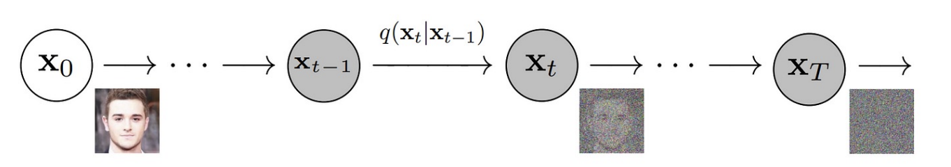
$\mathbf{Fig\ 1.}$ Forward diffusion process (source: [2])

A notable property is that given $\mathbf{x}_0$, $\mathbf{x}_t$ at any arbitrary timestep $t$ it can be directly sampled in closed form by reparameterization. By letting \(\alpha_t = 1 - \beta_t\) and \(\bar{\alpha}_t = \prod_{i=1}^t \alpha_i\),

\[\begin{aligned} \mathbf{x}_t &= \sqrt{\alpha_t} \color{blue}{\mathbf{x}_{t-1}} + \sqrt{1 - \alpha_t} \boldsymbol{\epsilon}_{t-1} & \text{ where } \boldsymbol{\epsilon} \sim \mathcal{N}(\mathbf{0}, \mathbf{I}) \\ & = \sqrt{\alpha_t} (\color{blue}{\sqrt{\alpha_{t-1}} \mathbf{x}_{t-2} + \sqrt{1 - \alpha_{t-1}} \boldsymbol{\epsilon}_{t-2}}) + \sqrt{1 - \alpha_t} \boldsymbol{\epsilon}_{t-1} \\ & = \sqrt{\alpha_t \alpha_{t-1}} \mathbf{x}_{t-2} + \color{red}{\sqrt{\alpha_t (1 - \alpha_{t-1})} \boldsymbol{\epsilon}_{t-2} + \sqrt{1 - \alpha_{t}} \boldsymbol{\epsilon}_{t-1}} \\ & = \sqrt{\alpha_t \alpha_{t-1}} \mathbf{x}_{t-2} + \color{red}{\sqrt{1 - \alpha_t \alpha_{t-1}} \bar{\boldsymbol{\epsilon}}_{t-2}} & \because \mathbf{x}_1 + \mathbf{x}_2 \sim \mathcal{N}(\mu_1 + \mu_2, (\sigma_1^2 + \sigma_2^2)\mathbf{I}) \\ & = \dots \\ & = \sqrt{\bar{\alpha}_t}\mathbf{x}_0 + \sqrt{1 - \bar{\alpha}_t}\boldsymbol{\epsilon} \\ & \therefore q(\mathbf{x}_t \vert \mathbf{x}_0) = \mathcal{N}(\sqrt{\bar{\alpha}_t} \mathbf{x}_0, (1 - \bar{\alpha}_t)\mathbf{I}) \end{aligned}\]

Note that \(q(\mathbf{x}_t \vert \mathbf{x}_0)\) becomes the unit Gaussian (prior distribution) when \(\sqrt{\bar{\alpha}_t} \mathbf{x}_0 = 0\). Therefore while $\beta_t > 0$ is small, \(\sqrt{\bar{\alpha}_t}\) converges to $0$ when $T \to \infty$.

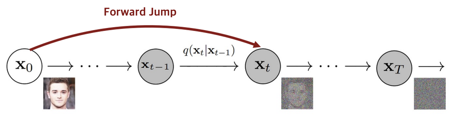
$\mathbf{Fig\ 2.}$ Forward Jump (source: [2])

Parametrization of $\beta_t$

$\beta_t$ can be learned or held constant as hyperparameters, but the expressiveness of the reverse process is enough by the choice of Gaussian conditionals in \(p_\theta (\mathbf{x}_{t−1} | \mathbf{x}_t)\), because of the mathematical fact from W. Feller, 1949 that both processes have the same functional form when $\beta_t$ are small. And the practical choice of $\beta_t$’s employed by Ho et al. 2020 is the linear interpolation from $\beta_1 = 10^{-4}$ to $\beta_T = 0.02$.

Reverse Process (Target → Data)

The reverse process maps the target distribution \(p(\mathbf{x} _T) \sim \mathcal{N}(\mathbf{0}, \mathbf{I})\) to the data distribution \(q(\mathbf{x}_0)\) and is defined as another Markov chain with learned Gaussian transitions $p_\theta (\mathbf{x}_{t-1} | \mathbf{x}_t)$ over timestep $t = T, \cdots, 1$:

\[\begin{aligned} p_\theta(\mathbf{x}_{t-1} \vert \mathbf{x}_t) = \mathcal{N}(\mathbf{x}_{t-1}; \boldsymbol{\mu}_\theta(\mathbf{x}_t, t), \boldsymbol{\Sigma}_\theta(\mathbf{x}_t, t) = \sigma_t^2 \mathbf{I}) \end{aligned} \\ \begin{aligned} p_{\theta} (\mathbf{x}_{0:T}) = \left(\prod_{t=1}^T p_{\theta} (\mathbf{x}_{t-1} | \mathbf{x}_t ) \right) p(\mathbf{x}_T), \quad p_{\theta} (\mathbf{x}_0) = \int p_{\theta} (\mathbf{x}_{0: T}) d\mathbf{x}_{1:T} \end{aligned}\]

Note that \(\boldsymbol{\Sigma}_\theta(\mathbf{x}_t, t)\) is not trained and fixed to time dependent constants. Practically, Ho et al. 2020 selects both \(\sigma^2_t = \beta_t\) and \(\sigma^2_t = \tilde{\beta_t} = \frac{1 - \bar{\alpha}_{t-1}}{1-\bar{\alpha}_{t}} \beta_t\).

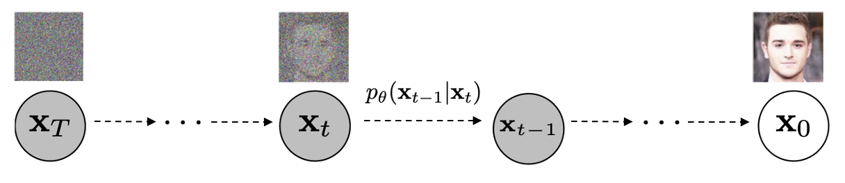
$\mathbf{Fig\ 3.}$ Reverse process (source: [2])

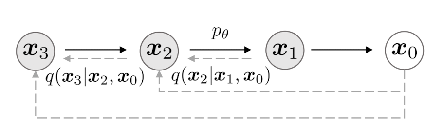
It has to be learned because although the reverse transition \(q(\mathbf{x}_{t-1} \mid \mathbf{x}_t)\) can be approximated as a Gaussian when $\beta_t$ is small, we cannot directly compute the distribution. But one should note that it is feasible when it is additionally conditioned on \(\mathbf{x}_0\). The closed form of \(q(\mathbf{x}_{t-1} \mid \mathbf{x}_t, \mathbf{x}_0)\) is derived as follows:

\[\begin{aligned} q(\mathbf{x}_{t-1} \vert \mathbf{x}_t, \mathbf{x}_0) &= q(\mathbf{x}_t \vert \mathbf{x}_{t-1}, \mathbf{x}_0) \frac{ q(\mathbf{x}_{t-1} \vert \mathbf{x}_0) }{ q(\mathbf{x}_t \vert \mathbf{x}_0) } \\ &\propto \exp \Big(-\frac{1}{2} \big(\frac{(\mathbf{x}_t - \sqrt{\alpha_t} \mathbf{x}_{t-1})^2}{\beta_t} + \frac{(\mathbf{x}_{t-1} - \sqrt{\bar{\alpha}_{t-1}} \mathbf{x}_0)^2}{1-\bar{\alpha}_{t-1}} - \frac{(\mathbf{x}_t - \sqrt{\bar{\alpha}_t} \mathbf{x}_0)^2}{1-\bar{\alpha}_t} \big) \Big) \\ &= \exp \Big(-\frac{1}{2} \big(\frac{\mathbf{x}_t^2 - 2\sqrt{\alpha_t} \mathbf{x}_t \color{blue}{\mathbf{x}_{t-1}} \color{black}{+ \alpha_t} \color{red}{\mathbf{x}_{t-1}^2} }{\beta_t} + \frac{ \color{red}{\mathbf{x}_{t-1}^2} \color{black}{- 2 \sqrt{\bar{\alpha}_{t-1}} \mathbf{x}_0} \color{blue}{\mathbf{x}_{t-1}} \color{black}{+ \bar{\alpha}_{t-1} \mathbf{x}_0^2} }{1-\bar{\alpha}_{t-1}} - \frac{(\mathbf{x}_t - \sqrt{\bar{\alpha}_t} \mathbf{x}_0)^2}{1-\bar{\alpha}_t} \big) \Big) \\ &\propto \exp\Big( -\frac{1}{2} \big((\color{red}{\frac{\alpha_t}{\beta_t} + \frac{1}{1 - \bar{\alpha}_{t-1}}}) \mathbf{x}_{t-1}^2 - (\color{blue}{\frac{2\sqrt{\alpha_t}}{\beta_t} \mathbf{x}_t + \frac{2\sqrt{\bar{\alpha}_{t-1}}}{1 - \bar{\alpha}_{t-1}} \mathbf{x}_0}) \mathbf{x}_{t-1} \color{black}{\big) \Big)} \end{aligned}\]

Note that it is a form of Gaussian with regard to $\mathbf{x}_{t-1}$. Thus, the mean and variance of distribution can be computed:

\[\begin{aligned} q(\mathbf{x}_{t−1} | \mathbf{x}_t, \mathbf{x}_0) = \mathcal{N} (\tilde{\boldsymbol{\mu}} (\mathbf{x}_t, \mathbf{x}_0), \tilde{\beta}_t \mathbf{I}) \end{aligned}\]

where

\[\begin{aligned} \tilde{\beta}_t & = \color{red}{1/(\frac{\alpha_t}{\beta_t} + \frac{1}{1 - \bar{\alpha}_{t-1}})} = 1 /(\frac{\alpha_t - \bar{\alpha}_t + \beta_t}{\beta_t(1 - \bar{\alpha}_{t-1})}) = \frac{1 - \bar{\alpha}_{t-1}}{1 - \bar{\alpha}_t} \cdot \beta_t \\ \tilde{\boldsymbol{\mu}} (\mathbf{x}_t, \mathbf{x}_0) & = (\frac{\sqrt{\alpha_t}}{\beta_t} \mathbf{x}_t + \frac{\sqrt{\bar{\alpha}_{t-1} }}{1 - \bar{\alpha}_{t-1}} \mathbf{x}_0)/\color{red}{(\frac{\alpha_t}{\beta_t} + \frac{1}{1 - \bar{\alpha}_{t-1}})} \\ & = (\frac{\sqrt{\alpha_t}}{\beta_t} \mathbf{x}_t + \frac{\sqrt{\bar{\alpha}_{t-1} }}{1 - \bar{\alpha}_{t-1}} \mathbf{x}_0) \color{red}{\frac{1 - \bar{\alpha}_{t-1}}{1 - \bar{\alpha}_t} \cdot \beta_t} \\ &= \frac{\sqrt{\alpha_t}(1 - \bar{\alpha}_{t-1})}{1 - \bar{\alpha}_t} \mathbf{x}_t + \frac{\sqrt{\bar{\alpha}_{t-1}}\beta_t}{1 - \bar{\alpha}_t} \mathbf{x}_0 \\ & = \frac{1}{\sqrt{\alpha_t}} \left( \mathbf{x}_t - \frac{1 - \alpha_t}{\sqrt{1 - \bar{\alpha}_t}} \boldsymbol{\epsilon}_t \right) = \tilde{\boldsymbol{\mu}} (\mathbf{x}_t, \boldsymbol{\epsilon}_t) & \because \mathbf{x}_t = \sqrt{\bar{\alpha}_t} \mathbf{x}_0 + \sqrt{1 - \bar{\alpha}_t} \boldsymbol{\epsilon}_t \end{aligned}\]

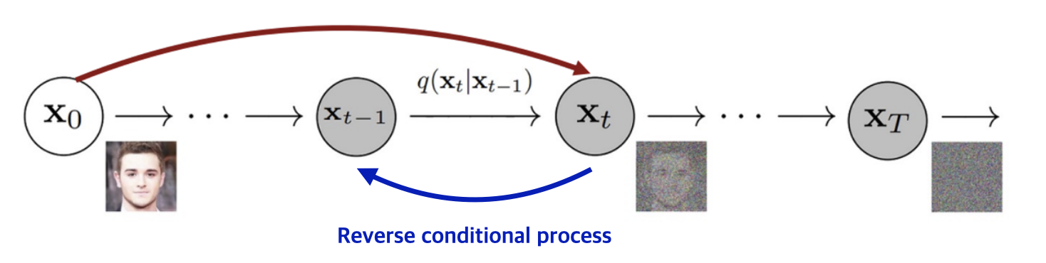
$\mathbf{Fig\ 4.}$ Reverse process conditioned on $\mathbf{x}_0$ (source: [2])

Parameterization of $\boldsymbol{\Sigma}_{\theta}$

The above discussion is based on when $\boldsymbol{\Sigma} _{\theta}(\mathbf{x} _t,t)$ is not trained and fixed to time dependent constants. Ho et al. 2020 selects both \(\sigma^2_t = \beta_t\) and \(\sigma^2_t = \tilde{\beta_t} = \frac{1 - \bar{\alpha}_{t-1}}{1-\bar{\alpha}_{t}} \beta_t\) since the authors observed that learned covariance $\boldsymbol{\Sigma} _{\theta}$ leads to unstable training with bad sample quality. Note that these two choices don’t affect sample quality as they are almost equal except near $t = 0$.

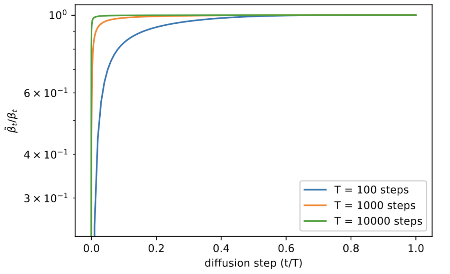
$\mathbf{Fig\ 4.}$ The ratio $\tilde{\beta_t}/\beta_t$ for every diffusion step (source: [3])

Training Loss

For training, it optimizes the variational lower bound:

$\color{red}{\mathbf{Theorem.}}$ $$ \begin{aligned} \mathbb{E}_{q(\mathbf{x}_0)} [- \log p_{\theta} (\mathbf{x}_0)] \leq \mathbb{E}_{q(\mathbf{x}_{0:T})} \left[ - \log \frac{p_\theta (\mathbf{x}_{0:T})}{q(\mathbf{x}_{1:T} | \mathbf{x}_0)} \right] := L \end{aligned} $$

$\mathbf{Proof.}$

We use the non-negativity of KL divergence:

\[\begin{aligned} - \log p_{\theta} (\mathbf{x}_0) & \leq - \log p_{\theta} (\mathbf{x}) + \text{KL}(q(\mathbf{x}_{1:T} | \mathbf{x}_0) \Vert p_{\theta} (\mathbf{x}_{1:T} | \mathbf{x}_0)) \\ & = - \log p_{\theta} (\mathbf{x}) + \mathbb{E}_{q(\mathbf{x}_{1:T} | \mathbf{x}_0)} \left[ \log \frac{q(\mathbf{x}_{1:T} | \mathbf{x}_0)}{p_{\theta} (\mathbf{x}_{0:T})} + \log p_{\theta} (\mathbf{x}_0) \right] \\ & = \mathbb{E}_{q(\mathbf{x}_{1:T} | \mathbf{x}_0)} \left[ \log \frac{q(\mathbf{x}_{1:T} | \mathbf{x}_0)}{p_{\theta} (\mathbf{x}_{0:T})} \right] \end{aligned}\] \[\tag*{$\blacksquare$}\]

And $L$ can be further extended into the combination of tractable terms:

$\color{red}{\mathbf{Theorem.}}$ $$ \begin{aligned} L = \mathbb{E}_{q(\mathbf{x}_{0:T})} [\underbrace{\text{KL}(q(\mathbf{x}_T \vert \mathbf{x}_0) \parallel p_\theta(\mathbf{x}_T))}_{L_T: \text{ regularization }} + \sum_{t=2}^T \underbrace{\text{KL}(q(\mathbf{x}_{t-1} \vert \mathbf{x}_t, \mathbf{x}_0) \parallel p_\theta(\mathbf{x}_{t-1} \vert\mathbf{x}_t))}_{L_{t-1} : \text{ denoising process }} \underbrace{- \log p_\theta(\mathbf{x}_0 \vert \mathbf{x}_1)}_{L_0: \text{ reconstruction }} ] \end{aligned} $$

$\mathbf{Proof.}$

The proof is nothing more than expansion of joint probability.

\[\begin{aligned} L & := \mathbb{E}_{q(\mathbf{x}_{0:T})} \left[ \log\frac{q(\mathbf{x}_{1:T}\vert\mathbf{x}_0)}{p_\theta(\mathbf{x}_{0:T})} \right] \\ & = \mathbb{E}_{q(\mathbf{x}_{0:T})} \left[ \log\frac{\prod_{t=1}^T q(\mathbf{x}_{t} \vert \mathbf{x}_{t-1})}{p_\theta(\mathbf{x}_{T}) \prod_{t=1}^T p_{\theta} (\mathbf{x}_{t-1} \vert \mathbf{x}_t)} \right] \\ & = \mathbb{E}_{q(\mathbf{x}_{0:T})} \left[ - \log p_{\theta} (\mathbf{x}_T) + \sum_{t=1}^T \log \frac{q (\mathbf{x}_t \vert \mathbf{x}_{t-1})}{p_{\theta} (\mathbf{x}_{t-1} \vert \mathbf{x}_t)} \right] \\ & = \mathbb{E}_{q(\mathbf{x}_{0:T})} \left[ - \log p_{\theta} (\mathbf{x}_T) + \sum_{t=2}^T \log \left( \frac{q (\mathbf{x}_{t-1} \vert \mathbf{x}_{t}, \mathbf{x}_0)}{p_{\theta} (\mathbf{x}_{t-1} \vert \mathbf{x}_t)} \cdot \frac{q(\mathbf{x}_t \vert \mathbf{x}_0)}{q(\mathbf{x}_{t-1} \vert \mathbf{x}_0)} \right) + \log \frac{q (\mathbf{x}_1 \vert \mathbf{x}_{0})}{p_{\theta} (\mathbf{x}_{0} \vert \mathbf{x}_{1})} \right] \\ & = \mathbb{E}_{q(\mathbf{x}_{0:T})} \left[ - \log p_{\theta} (\mathbf{x}_T) + \sum_{t=2}^T \log \frac{q (\mathbf{x}_{t-1} \vert \mathbf{x}_{t}, \mathbf{x}_0)}{p_{\theta} (\mathbf{x}_{t-1} \vert \mathbf{x}_t)} + \sum_{t=2}^T \log \frac{q(\mathbf{x}_t \vert \mathbf{x}_0)}{q(\mathbf{x}_{t-1} \vert \mathbf{x}_0)} + \log \frac{q (\mathbf{x}_1 \vert \mathbf{x}_{0})}{p_{\theta} (\mathbf{x}_{0} \vert \mathbf{x}_{1})} \right] \\ & = \mathbb{E}_{q(\mathbf{x}_{0:T})} \left[ - \log p_{\theta} (\mathbf{x}_T) + \sum_{t=2}^T \log \frac{q (\mathbf{x}_{t-1} \vert \mathbf{x}_{t}, \mathbf{x}_0)}{p_{\theta} (\mathbf{x}_{t-1} \vert \mathbf{x}_t)} + \log \frac{q(\mathbf{x}_T \vert \mathbf{x}_0)}{q(\mathbf{x}_{1} \vert \mathbf{x}_0)} + \log \frac{q (\mathbf{x}_1 \vert \mathbf{x}_{0})}{p_{\theta} (\mathbf{x}_{0} \vert \mathbf{x}_{1})} \right] \\ & = \mathbb{E}_{q(\mathbf{x}_{0:T})} \left[ \log \frac{q (\mathbf{x}_1 \vert \mathbf{x}_{0})}{p_{\theta} (\mathbf{x}_T)} + \sum_{t=2}^T \log \frac{q (\mathbf{x}_{t-1} \vert \mathbf{x}_{t}, \mathbf{x}_0)}{p_{\theta} (\mathbf{x}_{t-1} \vert \mathbf{x}_t)} + \log \frac{q(\mathbf{x}_T \vert \mathbf{x}_0)}{q(\mathbf{x}_{1} \vert \mathbf{x}_0)} - \log p_{\theta} (\mathbf{x}_{0} \vert \mathbf{x}_{1}) \right] \end{aligned}\] \[\tag*{$\blacksquare$}\]

Parametrization of $L_t$

The novelty of DDPM comes from the parametrization of loss terms. Note that $L_T$ is constant with respect to $\theta$ as $\beta_t$ is time-dependent constant. The final term in loss $L_0$​ closely resembles the reconstruction term employed in the Variational Autoencoder (VAE), albeit appearing in slightly varied contexts. When approximating the data distribution \(\mathbf{x} _0 \sim p(\mathbf{x} _0)\), remember that the ultimate optimization objective of a VAE comprises two components: the KL divergence between the latent prior and posterior, and the reconstruction term \(\mathbb{E}_{z\sim q(z \vert x_0)} [\log p(x_0 \vert z)]\). But in DDPM, instead of modeling $p(x_0 \vert z)$ as a gaussian, which assumes \(\mathbf{x}_0\) is continuous data point, the author design a separate discrete decoder to model the distribution \(p(\mathbf{x}_0 \vert \mathbf{x}_1)\) (\(\mathbf{x}_1\) in DDPM is equivalent to $z$ in VAE) with discrete log-likelihoods, since \(\mathbf{x}_0\) is dicrete image data whose values lie in the range $[0, 255]$. Originally, they designed an independent discrete decoder derived from the Gaussian $\mathcal{N}(\boldsymbol{\mu}_{\theta} (\mathbf{x}_1, 1), \sigma_1^2 \mathbf{I})$:

\[\begin{aligned} p_\theta\left(\mathbf{x}_0 \mid \mathbf{x}_1\right) & =\prod_{i=1}^D \int_{\delta_{-}\left(x_0^i\right)}^{\delta_{+}\left(x_0^i\right)} \mathcal{N}\left(x ; \boldsymbol{\mu}_\theta^i\left(\mathbf{x}_1, 1\right), \sigma_1^2\right) d x \\ \delta_{+}(x) & =\left\{\begin{array}{ll} \infty & \text { if } x=1 \\ x+\frac{1}{255} & \text { if } x<1 \end{array} \quad \delta_{-}(x)= \begin{cases}-\infty & \text { if } x=-1 \\ x-\frac{1}{255} & \text { if } x>-1\end{cases} \right. \end{aligned}\]

But the authors make simplification by replacing the integral by the Gaussian probability density function times the bin width, ignoring $\sigma_1$ and edge effects \(p_{\theta} (\mathbf{x}_0 \vert \mathbf{x}_1) = \frac{1}{\sqrt{2\pi}\sigma_1} \exp \left(\frac{\mathbf{x}_0 - \boldsymbol{\mu}_\theta (\mathbf{x}_1, 1)}{-2\sigma_1^2}\right) \times \frac{2}{255}\) where

\[\begin{aligned} \log p_{\theta} (\mathbf{x}_0 \vert \mathbf{x}_1) = \frac{-1}{2\sigma_1^2} \lVert \mathbf{x}_0 - \boldsymbol{\mu}_\theta (\mathbf{x}_1, 1) \rVert^2 + C. \end{aligned}\]

From \(\mathbf{x}_0 = \frac{1}{\sqrt{\tilde{\alpha}_1}} (\mathbf{x}_1 - \sqrt{1 - \tilde{\alpha}_1} \boldsymbol{\epsilon})\) and \(\boldsymbol{\mu}_\theta (\mathbf{x}_1, 1) = \frac{1}{\sqrt{\tilde{\alpha}_1}} (\mathbf{x}_1 - \sqrt{1 - \tilde{\alpha}_1} \boldsymbol{\epsilon}_{\theta} (\mathbf{x}_1, 1))\), finally we have

\[\begin{aligned} L_0 = \frac{1 - \alpha_1}{2\sigma_1^2 \alpha_1} \lVert \boldsymbol{\epsilon} - \boldsymbol{\epsilon}_{\theta} (\mathbf{x}_1, 1) \rVert^2. \end{aligned}\]

Now let’s turn our attention to $t \geq 1$ case. Recall the KL divergence between two $d$-dimensional Gaussians:

\[\begin{aligned} \text{KL} (\mathcal{N} (\boldsymbol{\mu}_1, \boldsymbol{\Sigma}_1) \Vert \mathcal{N} (\boldsymbol{\mu}_2, \boldsymbol{\Sigma}_2)) = \frac{1}{2} \left[ \text{tr}\left(\boldsymbol{\Sigma}_2^{-1} \boldsymbol{\Sigma}_1 \right) + (\boldsymbol{\mu}_2 - \boldsymbol{\mu}_1)^\top \boldsymbol{\Sigma}_2^{-1} (\boldsymbol{\mu}_2 - \boldsymbol{\mu}_1) - d + \log \frac{\det \boldsymbol{\Sigma}_2}{\det \boldsymbol{\Sigma}_1} \right] \end{aligned}\]

From

\[\begin{aligned} p_\theta(\mathbf{x}_{t-1} \vert \mathbf{x}_t) = \mathcal{N}(\boldsymbol{\mu}_\theta(\mathbf{x}_t, t), \boldsymbol{\Sigma}_\theta(\mathbf{x}_t, t) = \sigma_t^2 \mathbf{I}) \end{aligned} \\ \begin{aligned} q(\mathbf{x}_{t−1} | \mathbf{x}_t, \mathbf{x}_0) = \mathcal{N} \left(\tilde{\boldsymbol{\mu}} (\mathbf{x}_t, \boldsymbol{\epsilon}_t) = \frac{1}{\sqrt{\alpha_t}} \left( \mathbf{x}_t - \frac{1 - \alpha_t}{\sqrt{1 - \bar{\alpha}_t}} \boldsymbol{\epsilon}_t \right), \frac{1-\bar{\alpha}_{t-1}}{1-\bar{\alpha}_t} \cdot \beta_t \right) \end{aligned}\]

the loss term $L_t$ is parameterized to minimize the difference from the forward process posterior mean $\tilde{\boldsymbol{\mu}} (\mathbf{x}_t, \boldsymbol{\epsilon}_t)$ by considering only terms related to $\theta$:

\[\begin{aligned} L_{t-1} = \mathbb{E}_{q} \left[ \frac{1}{2 \sigma_t^2} \lVert \tilde{\boldsymbol{\mu}} (\mathbf{x}_t, \boldsymbol{\epsilon}_t) - \boldsymbol{\mu}_{\theta} (\mathbf{x}_t, t) \rVert^2 \right] + C \end{aligned}\]

It implies that \(\boldsymbol{\mu}_{\theta}\) must predict \(\tilde{\boldsymbol{\mu}}\). Hence the parametrization \(\boldsymbol{\mu}_{\theta}(\mathbf{x}_t, t) = \frac{1}{\sqrt{\alpha_t}} \left( \mathbf{x}_t - \frac{1 - \alpha_t}{\sqrt{1 - \bar{\alpha}_t}} \boldsymbol{\epsilon}_\theta (\mathbf{x}_t, t) \right)\) is straightforward. Thus $L_t$ is further simplified to

\[\begin{aligned} L_t = \mathbb{E}_{\mathbf{x}_0, \boldsymbol{\epsilon}}\left[\frac{\beta_t^2}{2 \sigma_t^2 \alpha_t\left(1-\bar{\alpha}_t\right)}\left\|\boldsymbol{\epsilon}-\boldsymbol{\epsilon}_\theta\left(\mathbf{x}_t = \sqrt{\bar{\alpha}_t} \mathbf{x}_0+\sqrt{1-\bar{\alpha}_t} \boldsymbol{\epsilon}, t\right)\right\|^2\right] \end{aligned}\]

Empirically, Ho et al. 2020 found it beneficial to sample quality to train on the simplified objective without the weight that unifies $L_t$ for $t = 0, 1, \cdots, T-1$:

\[\begin{aligned} L_{\text{simple}} = \mathbb{E}_{t \sim U[1, T], \mathbf{x}_0, \boldsymbol{\epsilon}} \left[\left\|\boldsymbol{\epsilon}-\boldsymbol{\epsilon}_\theta\left(\sqrt{\bar{\alpha}_t} \mathbf{x}_0+\sqrt{1-\bar{\alpha}_t} \boldsymbol{\epsilon}, t\right)\right\|^2\right] \end{aligned}\]

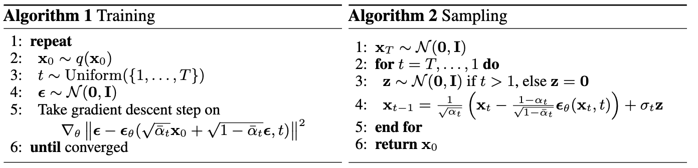
$\mathbf{Fig\ 5.}$ Pseudocode of DDPM (source: [2])

Connection with NCSN

Recall the objective of NCSN $\mathbf{s}_{\theta} (\mathbf{x})$ that estimates the score of data density:

\[\begin{aligned} \mathbb{E}_{\tilde{\mathbf{x}} \sim \mathcal{N}\left(\mathbf{x}, \sigma^2 I\right)}\left[\left\|\mathbf{s}_{\boldsymbol{\theta}}(\tilde{\mathbf{x}}, \sigma)+\frac{\tilde{\mathbf{x}}-\mathbf{x}}{\sigma^2}\right\|_2^2\right] \end{aligned}\]

In diffusion formulation, the score network can be modeled for denoising score matching over multiple noise scales indexed by $t$, \(\mathbf{s}_{\theta} (\mathbf{x}_t, t)\) approximating \(\nabla_{\mathbf{x}_t} \log q(\mathbf{x}_t)\). With \(q(\mathbf{x}_t \vert \mathbf{x}_0) \sim \mathcal{N}(\sqrt{\bar{\alpha}_t} \mathbf{x}_0, (1 - \bar{\alpha}_t)\mathbf{I})\) we have

\[\begin{aligned} \nabla_{\mathbf{x}_t} \log q(\mathbf{x}_t) & = \mathbb{E}_{q(\mathbf{x}_0)} [\nabla_{\mathbf{x}_t} q(\mathbf{x}_t \vert \mathbf{x}_0)] \\ & = \mathbb{E}_{q(\mathbf{x}_0)} \Big[ - \frac{\boldsymbol{\epsilon}}{\sqrt{1 - \bar{\alpha}_t}} \Big] & \because \nabla_\mathbf{x} \log \mathcal{N}(\boldsymbol{\mu}, \sigma^2 \mathbf{I}) = - \frac{\mathbf{x} - \boldsymbol{\mu}}{\sigma^2} = - \frac{\boldsymbol{\epsilon}}{\sigma} \\ & = - \frac{\boldsymbol{\epsilon}}{\sqrt{1 - \bar{\alpha}_t}} \end{aligned}\]

Therefore, the score network of diffusion approximates $\nabla_{\mathbf{x}_t} \log q(\mathbf{x}_t)$ by noise prediction: \(\mathbf{s}_{\theta} (\mathbf{x}_t, t) = - \frac{\boldsymbol{\epsilon}_{\theta} (\mathbf{x}_t, t)}{\sqrt{1 - \bar{\alpha}_t}}\).

Recall the annealed Langevin dynamics used for inference of NCSN:

\[\begin{aligned} \tilde{\mathbf{x}}_{t-1} \leftarrow \tilde{\mathbf{x}}_{t} + \frac{\alpha_i}{2} \mathbf{s}_{\boldsymbol{\theta}} (\tilde{\mathbf{x}}_{t}, \sigma_i) + \sqrt{\alpha_i} \mathbf{z}_t \end{aligned}\]

Note that the timestep flow of NCSN and diffusion are reversed. The sampling of DDPM resembles Langevin dynamics that samples the next data point $\mathbf{x} _{t-1}$ with the combination of previous data point $\mathbf{x} _t$, score $\boldsymbol{\epsilon} _{\theta} (\mathbf{x} _t, t)$, and random noise $\mathbf{z}$.

Improved DDPM

At the first time, it was unclear that DDPMs can achieve log-likelihoods competitive with other likelihood-based models such as autoregressive models and VAEs, and how well DDPMs scale to datasets with higher diversity such as ImageNet instead of CIFAR-10. Nichol & Dhariwal et al. 2021

Parametrization of $\beta_t$

Nichol & Dhariwal et al. 2021 proposed a different noise schedule

\[\begin{aligned} \beta_t = \text{clip}(1-\frac{\bar{\alpha}_t}{\bar{\alpha}_{t-1}}, 0.999) \quad\bar{\alpha}_t = \frac{f(t)}{f(0)}\quad\text{where }f(t)=\cos\Big(\frac{t/T+s}{1+s}\cdot\frac{\pi}{2}\Big)^2 \end{aligned}\]

Parametrization of $\boldsymbol{\Sigma}_{\theta}$

Nichol & Dhariwal et al. 2021 proposed to set $\boldsymbol{\Sigma}_{\theta}$ as a learnable parameter that interpolates $\beta_t$ and $\tilde{\beta}_t$ in log domain by extending the model to predict a weight vector $\mathbf{v}$:

\[\begin{aligned} \boldsymbol{\Sigma}_\theta(\mathbf{x}_t, t) = \exp(\mathbf{v} \log \beta_t + (1-\mathbf{v}) \log \tilde{\beta}_t) \end{aligned}\]

Denoising Diffusion Implicit Models (DDIM)

Denoising diffusion probabilistic models have demonstrated the high quality of samples comparable to that of GANs, but it requires a few steps of Markov chain for denoising samples perturbed by various levels of Gaussian noise, which could have thousands of steps. This makes DDPMs much slower compared to GANs that only needs one pass through a network. For example, the author of Ho et al. 2020 explain that DDPM takes around 20 hours to sample 50K images of size $32 \times 32$ from a DDPM, but less than a minute to do so from a GAN on a NVIDIA 2080 Ti GPU. For larger images of size $256 \times 256$, it could take nearly 1000 hours.

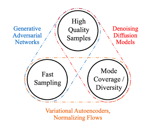
$\mathbf{Fig\ 6.}$ Generative learning trilemma (source: NVIDIA)

To enhance the efficiency, denoising diffusion implicit models (DDIMs), proposed by Song et al. 2021, generalize the Markovian forward process to non-Markovian, for which we are still able to design suitable reverse generative Markov chains. And also the authors maintain the resulting variational training objectives to have a shared surrogate objective used in DDPM. The goal of DDIM is to make a deterministic generative process while using the same noise prediction model trained for DDPM to accelerate generation speed.

Another approaches are still possible to speeding up diffusion models for images, for example embedding the images into a lower dimensional space, and then fit the diffusion model to the embeddings. This idea has been pursued in several papers including latent diffusion model (LDM), which we will discuss in the next post.

Non-Markovian Forward Process

From \(\mathbf{x}_1 + \mathbf{x}_2 \sim \mathcal{N}(\mu_1 + \mu_2, (\sigma_1^2 + \sigma_2^2) \mathbf{I})\) we have

\[\begin{aligned} \mathbf{x}_{t-1} & = \sqrt{\bar{\alpha}_{t-1}}\mathbf{x}_0 + \sqrt{1 - \bar{\alpha}_{t-1}}\boldsymbol{\epsilon}_{t-1} \\ & = \sqrt{\bar{\alpha}_{t-1}}\mathbf{x}_0 + \sqrt{1 - \bar{\alpha}_{t-1} - \sigma_t^2} \boldsymbol{\epsilon}_t + \sigma_t\boldsymbol{\epsilon} \\ & = \sqrt{\bar{\alpha}_{t-1}}\mathbf{x}_0 + \sqrt{1 - \bar{\alpha}_{t-1} - \sigma_t^2} \frac{\mathbf{x}_t - \sqrt{\bar{\alpha}_t}\mathbf{x}_0}{\sqrt{1 - \bar{\alpha}_t}} + \sigma_t\boldsymbol{\epsilon} \\ q_\sigma(\mathbf{x}_{t-1} \vert \mathbf{x}_t, \mathbf{x}_0) & = \mathcal{N}\left(\sqrt{\bar{\alpha}_{t-1}}\mathbf{x}_0 + \sqrt{1 - \bar{\alpha}_{t-1} - \sigma_t^2} \frac{\mathbf{x}_t - \sqrt{\bar{\alpha}_t}\mathbf{x}_0}{\sqrt{1 - \bar{\alpha}_t}}, \sigma_t^2 \mathbf{I}\right) \end{aligned}\]

Note that this coefficients are selected to match the marginals \(q_\sigma (\mathbf{x}_t \vert \mathbf{x}_0)\) match with DDPM. Then consider the following forward process with parameters \(\{ \bar{\alpha}_t \}\) and hyperparameter $\sigma_t$:

\[\begin{aligned} q_\sigma(\mathbf{x}_{1:T} \vert \mathbf{x}_0) = q_\sigma(\mathbf{x}_T \vert \mathbf{x}_0) \prod_{t=2}^T q_\sigma(\mathbf{x}_{t-1} \vert \mathbf{x}_t, \mathbf{x}_0) \end{aligned} \\ \begin{aligned} \text{ where } q_\sigma(\mathbf{x}_t \vert \mathbf{x}_0) = \mathcal{N}(\sqrt{\bar{\alpha}_t} \mathbf{x}_0, (1-\bar{\alpha}_t) \mathbf{I}) \end{aligned} \\ \begin{aligned} q_\sigma(\mathbf{x}_{t-1} \vert \mathbf{x}_t, \mathbf{x}_0) = \mathcal{N} \left( \sqrt{\bar{\alpha}_{t-1}} \mathbf{x}_0 + \sqrt{1 - \bar{\alpha}_{t-1} - \sigma_t^2} \cdot \frac{\mathbf{x}_t - \sqrt{\bar{\alpha}_t}\mathbf{x}_0}{\sqrt{1 - \bar{\alpha}_{t}}}, \sigma_t^2 \mathbf{I} \right) \end{aligned}\]

Then the forward non-Markovian transition is derived from Bayes’ rule:

\[\begin{aligned} q(\mathbf{x}_t \vert \mathbf{x}_{t-1}, \mathbf{x}_0) = \frac{q(\mathbf{x}_{t-1} \vert \mathbf{x}_t, \mathbf{x}_0) q(\mathbf{x}_t \vert \mathbf{x}_0)}{q(\mathbf{x}_{t-1} \vert \mathbf{x}_0)} \end{aligned}\]

$\mathbf{Fig\ 8.}$ Non-Markovian forward process (source: [4])

Note that when \(\sigma_t = \sqrt{\frac{1 - \bar{\alpha}_{t-1}}{1 - \bar{\alpha}_t}} \sqrt{1 - \frac{\bar{\alpha}_t}{\bar{\alpha}_{t-1}}}\) for all $t$, the forward process becomes Markovian . Another special case is $\sigma_t = 0$ for all $t$. Then the forward process becomes deterministic given \(\mathbf{x}_{t-1}\) and \(\mathbf{x}_0\), except for $t = 1$. This special case is named the denoising diffusion implicit model (DDIM). We will see why it is named like this below.

Modified Reverse Process

We define a trainable generative process \(p _{\theta}(\mathbf{x} _{0:T})\) where each \(p _{\theta}(\mathbf{x} _{t−1} \vert \mathbf{x} _t)\) leverages knowledge of \(q _{\sigma} (\mathbf{x} _{t−1} \vert \mathbf{x} _t, \mathbf{x} _0)\). For \(\mathbf{x}_t \sim q(\mathbf{x}_0)\) and noise \(\boldsymbol{\epsilon}_t\), recall that the noise prediction model \(\boldsymbol{\epsilon}_{\theta} (\mathbf{x}_t, t)\) in DDPM predict \(\boldsymbol{\epsilon}_t\) from \(\mathbf{x}_t\), without knowledge of data \(\mathbf{x}_0\). And from forward jump equation, it can then predict the denoised observation:

\[\begin{aligned} f_{\theta} (\mathbf{x}_t, t) := \frac{\mathbf{x}_t - \sqrt{1 - \bar{\alpha}_t} \cdot \boldsymbol{\epsilon}_{\theta} (\mathbf{x}_t, t)}{\sqrt{\bar{\alpha}_t}} \end{aligned}\]

Then we can then define the reverse process with a fixed prior $p_{\theta} (\mathbf{x}_T ) = \mathcal{N}(\mathbf{0}, \mathbf{I})$:

\[\begin{aligned} p_{\theta} (\mathbf{x}_{t-1} \vert \mathbf{x}_t) = \begin{cases} \mathcal{N}(f_{\theta} (\mathbf{x}_1, 1), \sigma_1^2 \mathbf{I}) & \text{ if } t = 1 \\ q_{\sigma} (\mathbf{x}_{t-1} \vert \mathbf{x}_t, f_{\theta} (\mathbf{x}_t, t)) & \text{ otherwise } \\ \end{cases} \end{aligned}\]

Intuitively, given a perturbed observation \(\mathbf{x}_t\), we first make a prediction of the corresponding \(\mathbf{x}_0\), and then use it to obtain a sample \(\mathbf{x}_{t−1}\) through the reverse conditional distribution \(q_{\sigma} (\mathbf{x}_{t−1} \vert \mathbf{x}_t, \mathbf{x}_0)\) that we have defined. For the case of $t = 1$, it adds the Gaussian noise with covariance \(\sigma_1^2 \mathbf{I}\) to ensure that the reverse process is supported everywhere.

Training Objective

We optimize $\theta$ via the following variational inference objective

\[\begin{aligned} & J_{\sigma} (\boldsymbol{\epsilon}_{\theta}) := \mathbb{E}_{\mathbf{x}_{0: T} \sim q_{\sigma} (\mathbf{x}_{0:T})} [\log q_{\sigma} (\mathbf{x}_{1:T} \vert \mathbf{x}_0) - \log p_{\theta} (\mathbf{x}_{0:T})] \\ = \; & \mathbb{E}_{\mathbf{x}_{0:T} \sim q_\sigma (\mathbf{x}_{0:T})} \left[ \log q_\sigma (\mathbf{x}_T \vert \mathbf{x}_0) + \sum_{t=2}^T \log q_{\sigma} (\mathbf{x}_{t-1} \vert \mathbf{x}_t, \mathbf{x}_0) - \sum_{t=1}^T \log p_{\theta} (\mathbf{x}_{t-1} \vert \mathbf{x}_t) - \log p_{\theta} (\mathbf{x}_T) \right] \end{aligned}\]

$\color{red}{\mathbf{Theorem.}}$ For a vector of positive coefficients $\gamma := [\gamma_1, \cdots, \gamma_T]$, define $$ \begin{aligned} L_\gamma (\boldsymbol{\epsilon}_\theta) := \sum_{t=1}^T \gamma_t \mathbb{E}_{\mathbf{x}_0 \sim q(\mathbf{x}_0), \boldsymbol{\epsilon} \sim \mathcal{N}(\mathbf{0}, \mathbf{I})} \left[ \lVert \boldsymbol{\epsilon} - \boldsymbol{\epsilon}_{\theta}(\mathbf{x}_t, t) \rVert_2^2 \right] \end{aligned} $$ For all $\sigma > \mathbf{0}$, there exists $\gamma \in \mathbb{R}_+^T$ and $C \in \mathbb{R}$ such that $$ \begin{aligned} J_\sigma = L_\gamma + C. \end{aligned} $$

$\mathbf{Proof.}$

From the definition of $J_\sigma$, we can discard the terms independent of $\theta$:

\[\begin{aligned} J_\sigma & := \mathbb{E}_{\mathbf{x}_{0:T} \sim q_\sigma (\mathbf{x}_{0:T})} \left[ \log q_\sigma (\mathbf{x}_T \vert \mathbf{x}_0) + \sum_{t=2}^T \log q_{\sigma} (\mathbf{x}_{t-1} \vert \mathbf{x}_t, \mathbf{x}_0) - \sum_{t=1}^T \log p_{\theta} (\mathbf{x}_{t-1} \vert \mathbf{x}_t) - \log p_{\theta} (\mathbf{x}_T) \right] \\ & \propto \mathbb{E}_{\mathbf{x}_{0:T} \sim q_\sigma (\mathbf{x}_{0:T})} \left[ \sum_{t=2}^T \text{KL}(q_{\sigma} (\mathbf{x}_{t-1} \vert \mathbf{x}_t, \mathbf{x}_0) \Vert p_{\theta} (\mathbf{x}_{t-1} \vert \mathbf{x}_t)) - \log p_{\theta} (\mathbf{x}_0 \vert \mathbf{x}_1) \right] \end{aligned}\]

Suppose the dimension of $\mathbf{x}_0$ to be $d$. Recall the KL divergence between two $d$-dimensional Gaussians:

\[\begin{aligned} \text{KL} (\mathcal{N} (\boldsymbol{\mu}_1, \boldsymbol{\Sigma}_1) \Vert \mathcal{N} (\boldsymbol{\mu}_2, \boldsymbol{\Sigma}_2)) = \frac{1}{2} \left[ \text{tr}\left(\boldsymbol{\Sigma}_2^{-1} \boldsymbol{\Sigma}_1 \right) + (\boldsymbol{\mu}_2 - \boldsymbol{\mu}_1)^\top \boldsymbol{\Sigma}_2^{-1} (\boldsymbol{\mu}_2 - \boldsymbol{\mu}_1) - d + \log \frac{\det \boldsymbol{\Sigma}_2}{\det \boldsymbol{\Sigma}_1} \right] \end{aligned}\]

For $t > 1$:

\[\begin{aligned} & \mathbb{E}_{\mathbf{x}_0, \mathbf{x}_t \sim q(\mathbf{x}_0, \mathbf{x}_t)} [ \text{KL}(q_{\sigma} (\mathbf{x}_{t-1} \vert \mathbf{x}_t, \mathbf{x}_0) \Vert p_{\theta} (\mathbf{x}_{t-1} \vert \mathbf{x}_t)) ] \\ = \; & \mathbb{E}_{\mathbf{x}_0, \mathbf{x}_t \sim q(\mathbf{x}_0, \mathbf{x}_t)} [ \text{KL}(q_{\sigma} (\mathbf{x}_{t-1} \vert \mathbf{x}_t, \mathbf{x}_0) \Vert q_\sigma (\mathbf{x}_{t-1} \vert \mathbf{x}_t, f_{\theta} (\mathbf{x}_t, t))) ] \\ \propto \; & \mathbb{E}_{\mathbf{x}_0, \mathbf{x}_t \sim q(\mathbf{x}_0, \mathbf{x}_t)} \left[ \frac{\lVert \mathbf{x}_0 - f_{\theta} (\mathbf{x}_t, t) \rVert_2^2}{2\sigma_t^2} \right] \\ = \; & \mathbb{E}_{\mathbf{x}_0 \sim q(\mathbf{x}_0), \boldsymbol{\epsilon} \sim \mathcal{N}(\mathbf{0}, \mathbf{I}), \mathbf{x}_t = \sqrt{\bar{\alpha}_t} \mathbf{x}_0 + \sqrt{1-\bar{\alpha}_t} \boldsymbol{\epsilon}} \left[ \frac{\lVert \frac{\mathbf{x}_t - \sqrt{1 - \bar{\alpha}_t \boldsymbol{\epsilon}}}{\sqrt{\bar{\alpha}_t}} - \frac{\mathbf{x}_t - \sqrt{1 - \bar{\alpha}_t} \boldsymbol{\epsilon}_{\theta} (\mathbf{x}_t, t)}{\sqrt{\bar{\alpha}_t}} \rVert_2^2}{2\sigma_t^2}\right] \\ & = \mathbb{E}_{\mathbf{x}_0 \sim q(\mathbf{x}_0), \boldsymbol{\epsilon} \sim \mathcal{N}(\mathbf{0}, \mathbf{I}), \mathbf{x}_t = \sqrt{\bar{\alpha}_t} \mathbf{x}_0 + \sqrt{1-\bar{\alpha}_t} \boldsymbol{\epsilon}} \left[ \frac{\lVert \boldsymbol{\epsilon} - \boldsymbol{\epsilon}_{\theta} (\mathbf{x}_t, t) \rVert_2^2}{2d\sigma_t^2}\right] \end{aligned}\]

For $t = 1$:

\[\begin{aligned} & \mathbb{E}_{\boldsymbol{x}_0, \boldsymbol{x}_1 \sim q\left(\boldsymbol{x}_0, \boldsymbol{x}_1\right)}\left[-\log p_\theta^{(1)}\left(\boldsymbol{x}_0 \mid \boldsymbol{x}_1\right)\right] \propto \mathbb{E}_{\boldsymbol{x}_0, \boldsymbol{x}_1 \sim q\left(\boldsymbol{x}_0, \boldsymbol{x}_1\right)}\left[\frac{\left\|\boldsymbol{x}_0-f_\theta^{(t)}\left(\boldsymbol{x}_1\right)\right\|_2^2}{2 \sigma_1^2}\right] \\ = \; & \mathbb{E}_{\boldsymbol{x}_0 \sim q\left(\boldsymbol{x}_0\right), \epsilon \sim \mathcal{N}(\mathbf{0}, \boldsymbol{I}), \boldsymbol{x}_1=\sqrt{\alpha_1} \boldsymbol{x}_0+\sqrt{1-\alpha_t \epsilon}}\left[\frac{\left\|\epsilon-\epsilon_\theta^{(1)}\left(\boldsymbol{x}_1\right)\right\|_2^2}{2 d \sigma_1^2 \alpha_1}\right] \end{aligned}\]

Therefore, by setting $\gamma_t = 1 / (2d \sigma_t^2 \bar{\alpha}_t)$ for all $t = 1, 2, \cdots, T$, we have

\[\begin{aligned} J_{\sigma} (\boldsymbol{\epsilon}_\theta) \propto \sum_{t=1}^T \frac{1}{2d \sigma_t^2 \bar{\alpha}_t} \mathbb{E} \left[ \lVert \boldsymbol{\epsilon}_t - \boldsymbol{\epsilon}_\theta (\mathbf{x}_t, t) \rVert_2^2 \right] = L_\gamma ( \boldsymbol{\epsilon}_\theta ). \end{aligned}\] \[\tag*{$\blacksquare$}\]

This theorem implies that non-Markovian inference process of DDIM, with parameters of the model \(\boldsymbol{\epsilon}_{\theta}^{(t)} = \boldsymbol{\epsilon}_{\theta}(\cdot, t)\) that are not shared across different $t$, eventually lead to the same surrogate objective function as DDPM \(L_{\mathbf{1}} = L_{\text{simple}}\). Hence the optimal solution of $J_\sigma$ is equvalent to that of $L_{\text{simple}}$.

Accelerating Sampling Process

From $p_\theta (\mathbf{x} _{1:T})$, we can generate a sample $\mathbf{x} _{t-1}$ from a sample $\mathbf{x} _t$ via:

\[\begin{aligned} \mathbf{x}_{t-1} & = \sqrt{\bar{\alpha}_{t-1}}\mathbf{x}_0 + \sqrt{1 - \bar{\alpha}_{t-1}}\boldsymbol{\epsilon}_{t-1} \\ & = \sqrt{\bar{\alpha}_{t-1}}\mathbf{x}_0 + \sqrt{1 - \bar{\alpha}_{t-1} - \sigma_t^2} \boldsymbol{\epsilon}_t + \sigma_t\boldsymbol{\epsilon} \\ & = \sqrt{\bar{\alpha}_{t-1}}\mathbf{x}_0 + \sqrt{1 - \bar{\alpha}_{t-1} - \sigma_t^2} \frac{\mathbf{x}_t - \sqrt{\bar{\alpha}_t}\mathbf{x}_0}{\sqrt{1 - \bar{\alpha}_t}} + \sigma_t\boldsymbol{\epsilon} \\ \therefore \mathbf{x}_{t-1} & = \sqrt{\bar{\alpha}_{t-1}} \underbrace{\left(\frac{\mathbf{x}_t-\sqrt{1-\bar{\alpha}_t} \boldsymbol{\epsilon}_\theta \left(\mathbf{x}_t, t\right)}{\sqrt{\bar{\alpha}_t}}\right)}_{\text {" predicted } \mathbf{x}_0 \text { " }}+\underbrace{\sqrt{1-\bar{\alpha}_{t-1}-\sigma_t^2} \cdot \boldsymbol{\epsilon}_\theta \left(\mathbf{x}_t, t\right)}_{\text {"direction pointing to } \mathbf{x}_t \text { " }}+\underbrace{\sigma_t \boldsymbol{\epsilon}_t}_{\text {random noise }} \end{aligned}\]

where \(\boldsymbol{\epsilon}_t \sim \mathcal{N} (\mathbf{0}, \mathbf{I})\) and we define \(\bar{\alpha}_0 := 1\). Note that when \(\sigma_t = \sqrt{(1 - \bar{\alpha}_{t-1})(1 - \bar{\alpha}_t)} \sqrt{1 - \bar{\alpha}_t / \bar{\alpha}_{t-1}} = \sqrt{\tilde{\beta}_t}\) for all $t$, the forward process becomes Markovian and the generation process becomes a DDPM. Hence, DDIM is actually a generalized version of DDPM. Another special case is \(\sigma_t = 0\) for all $t$. Then the coefficient before the random noise \(\boldsymbol{\epsilon}_t\) becomes zero, thus both the forward and reverse processes become not stochastic but deterministic processes. Although this case is not covered in the objective equation, we can always approximate it by making σt very small. And this special case is named as the denoising diffusion implicit model (DDIM) since it is an implicit probabilistic model trained with the DDPM objective (despite the forward process no longer being a diffusion). Hence, if we set \(\sigma_t = \eta \sqrt{(1 - \bar{\alpha}_{t-1})(1 - \bar{\alpha}_t)} \sqrt{1 - \bar{\alpha}_t / \bar{\alpha}_{t-1}} = \eta \sqrt{\tilde{\beta}_t}\), we can simply interpolate between DDIM ($\eta = 0$) and DDPM ($\eta = 1$).

And the formulation of DDIM enables the sampling with a subset of timesteps without changing the DDPM training objective, which can accelerate the sampling speed of diffusion model. Let \(\tau = \{ \tau_i \vert i = 1, 2, \cdots S \}\) be a sub-sequence of $[1, \cdots, T]$ of length $S$ and let \(\bar{\tau} = \{1, \cdots, T\} \setminus \tau\). Then we can consider the forward process to be factored as:

\[\begin{aligned} q_{\sigma, \tau} (\mathbf{x}_{1:T} \vert \mathbf{x}_0) = q_{\sigma, \tau} (\mathbf{x}_{\tau_S} \vert \mathbf{x}_0) \prod_{i=1}^S q_{\sigma, \tau} (\mathbf{x}_{\tau_{i-1}} \vert \mathbf{x}_{\tau_i}, \mathbf{x}_0) \prod_{t \in \bar{\tau}} q_{\sigma, \tau} (\mathbf{x}_t \vert \mathbf{x}_0) \end{aligned}\]

with

\[\begin{aligned} q_{\sigma, \tau} (\mathbf{x}_t \vert \mathbf{x}_0) = \mathcal{N}(\sqrt{\bar{\alpha}_t} \mathbf{x}_0, (1 - \bar{\alpha}_t) \mathbf{I}) \; \forall t \in \bar{\tau} \cup \{ T \} \end{aligned} \\ \begin{aligned} q_{\sigma, \tau} (\mathbf{x}_{\tau_{i-1}} \vert \mathbf{x}_{\tau_i}, \mathbf{x}_0) = \mathcal{N}(\sqrt{\bar{\alpha}_{\tau_{i-1}}} \mathbf{x}_0 + \sqrt{1 - \bar{\alpha}_{\tau_{i-1}} - \sigma_{\tau_i}^2} \cdot \frac{\mathbf{x}_{\tau_i} - \sqrt{\alpha_{\tau_i}} \mathbf{x}_0}{\sqrt{1 - \bar{\alpha}_{\tau_i}}}, \sigma_{\tau_i}^2 \mathbf{I}) \end{aligned}\]

where the coefficients are chosen such that

\[\begin{aligned} q_{\sigma, \tau} (\mathbf{x}_{\tau_i} \vert \mathbf{x}_0) = \mathcal{N} (\sqrt{\bar{\alpha}_{\tau_i}} \mathbf{x}_0, (1 - \bar{\alpha}_{\tau_i}) \mathbf{I}) \end{aligned}\]

i.e., the marginals match. Then the reverse process can be factored as

\[\begin{aligned} p_\theta\left(\boldsymbol{x}_{0: T}\right):=\underbrace{p_\theta\left(\boldsymbol{x}_T\right) \prod_{i=1}^S p_\theta^{\left(\tau_i\right)}\left(\boldsymbol{x}_{\tau_{i-1}} \mid \boldsymbol{x}_{\tau_i}\right)}_{\text {use to produce samples }} \times \underbrace{\prod_{t \in \bar{\tau}} p_\theta^{(t)}\left(\boldsymbol{x}_0 \mid \boldsymbol{x}_t\right)}_{\text {in variational objective }}. \end{aligned}\]

where only part of the models are being used to produce samples. And each reverse step becomes

\[\begin{aligned} \mathbf{x}_{\tau_{i-1}} & = \sqrt{\bar{\alpha}_{\tau_{i-1}}} \left(\frac{\mathbf{x}_{\tau_i}-\sqrt{1-\bar{\alpha}_{\tau_i}} \boldsymbol{\epsilon}_\theta \left(\mathbf{x}_{\tau_i}, t\right)}{\sqrt{\bar{\alpha}_{\tau_i}}}\right) \mathbf{x}_0 +\sqrt{1-\bar{\alpha}_{\tau_{i-1}}-\sigma_{\tau_i}^2} \cdot \boldsymbol{\epsilon}_\theta \left(\mathbf{x}_{\tau_i}, \tau_i \right)\mathbf{x}_{\tau_i} +\sigma_{\tau_i} \boldsymbol{\epsilon}_{\tau_i} \end{aligned}\]

$\mathbf{Fig\ 9.}$ Graphical model for accelerated generation, (source: [4])

• As the number of timesteps $S$ decreases, the sample quality gets worse.
• But, as $\sigma_{\tau_i}$ gets closer to zero (deterministic), the quality degradation is minimized.

$\mathbf{Fig\ 10.}$ FID scores on CIFAR10 and CelebA datasets by diffusion models of different setting of $\eta$.
DDIM ($\eta = 0.0$) and DDPM ($\eta = 1.0$, $\hat{\sigma}$). (source: [4])

Compared to DDPM, DDIM is able to:

Generate higher-quality samples using a much fewer number of steps.
Have “consistency” property since the generative process is deterministic, meaning that multiple samples conditioned on the same latent variable should have similar high-level features.
Because of the consistency, DDIM can do semantically meaningful interpolation in the latent variable.

Connection with Neural ODE

Reference

[1] Sohl-Dickstein et al. “Deep unsupervised learning using nonequilibrium thermodynamics.” ICML 2015.
[2] Ho et al. “Denoising Diffusion Probabilistic Models” NeurIPS 2020.
[3] Nichol and Dhariwal et al. “Improved denoising diffusion probabilistic models.” International Conference on Machine Learning. PMLR, 2021.
[4] Song et al. “Denoising diffusion implicit models”, ICML 2021.