[Generative Model] Latent Diffusion Model

Introduction

Latent Diffusion Model (LDM), proposed by Rombach et al. CVPR 2022, operates directly in the latent space of trained autoencoders, instead of pixel space to unburden the complexity for limited computational resources.

LDM is built on the analysis of trained diffusion models in pixel space. Learning in likelihood-based models can be broadly divided into two stages: the first stage is termed perceptual compression, where high-frequency details are removed, focusing on learning minimal semantic variation. In the second stage, the actual generative model comes into play, learning the semantic and conceptual composition of the data (term semantic compression). This implies that the most of pixels in an image contribute to perceptual details rather than semantics. As one can observe in the following figure, most bits of an image correspond to imperceptible details. While DMs suppress this semantically meaningless information on all pixels of image, it costs unnecessarily expensive computations. The idea of LDM is to address perceptual compression using an autoencoder rather than a DM to eliminate difficult-to-recognize details.

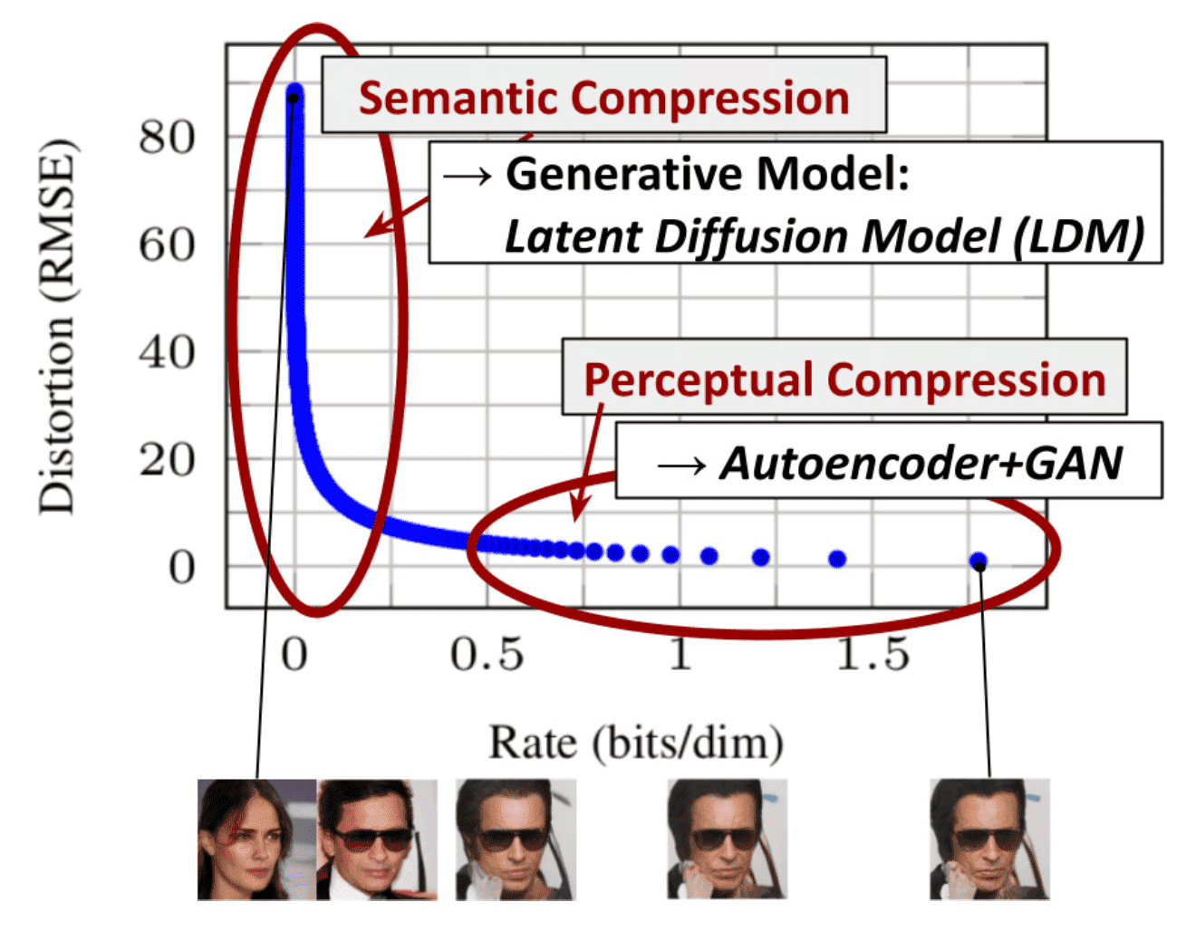
$\mathbf{Fig\ 1.}$ Perceptual and Semantic compression (Rombach et al. 2022)

Hence LDM aims to discover a low-dimensional space perceptually equivalent to the data space, and generates remaining sematic and conceptual pixels on that efficient space. This approach significantly decrease training and inference costs, offering high versatility as the trained low-dimensional space can be reused for multiple diffusion model trainings or to explore possibly completely different tasks.

Latent Diffusion Model

The perceptual compression process is built on on an autoencoder model with encoder $\mathcal{E}$ and decoder $\mathcal{D}$. Given an image $\mathbf{x} \in \mathbb{R}^{H \times W \times 3}$, an encoder $\mathcal{E}$ compresses $\mathbf{x}$ to 2D latent vector $\mathbf{z} = \mathcal{E}(\mathbf{x}) \in \mathbb{R}^{h \times w \times c}$, where the downsampling rate $f=H/h=W/w=2^m$ for some $m \in \mathbb{N}$. Then an decoder $\mathcal{D}$ reconstructs the images from the latent vector, giving $\tilde{\mathbf{x}} = \mathcal{D}(\mathbf{z})$. In order to avoid arbitrarily high-variance latent spaces, the authors experiment two different kinds of regularizations in autoencoder:

• KL-reg: a slight KL-penalty towards a standard normal distribution on the learned latent, similar to VAE.
• VQ-reg: uses a vector quantization layer within the decoder, like VQVAE but the quantization layer is absorbed by the decoder.

Details on Autoencoder

All autoencoder models are trained in an adversarial manner following VQGAN, such that a patch-based discriminator $D_{\psi}$ is optimized to differentiate original images from reconstructions $\mathcal{D}(\mathcal{E}(\mathbf{x}))$.

The regularization loss $L_{\text{reg}}$ is investigated by 2 different methods:

• KL-reg: a low-weighted KL loss term between \(q_\mathcal{E} (\mathbf{z} \vert \mathbf{x}) = \mathcal{N}(\mathcal{E}_{\mu}, \mathcal{E}_{\sigma^2})\) and a standard normal \(\mathcal{N}(\mathbf{0}, \mathbf{I})\) as in a standard VAE.
• VQ-reg: regularizing the latent space with a VQ layer by learning a codebook of $\vert \mathcal{Z} \vert$ different exemplars like VQ-VAE.

To obtain high-fidelity reconstructions the authors use a very small regularization for both scenarios, i.e. either weight the KL term by a factor ~ $10^{-6}$ or choose a high codebook dimensionality $\vert \mathcal{Z} \vert$. Then the final optimization loss can be written as follows:

\[\begin{aligned} L_{\text {Autoencoder }}=\min _{\mathcal{E}, \mathcal{D}} \max _\psi\left(L_{r e c}(x, \mathcal{D}(\mathcal{E}(x)))-L_{a d v}(\mathcal{D}(\mathcal{E}(x)))+\log D_\psi(x)+L_{r e g}(x ; \mathcal{E}, \mathcal{D})\right) \end{aligned}\]

Note that for training diffusion models on the learned latent space, we again distinguish two cases when learning $p(\mathbf{z})$ or $p(\mathbf{z} \vert y)$.

• KL-reg: sample \(\mathcal{z} = \mathcal{E}_\mu (\mathbf{x}) + \mathcal{E}_{\sigma} (\mathbf{x}) \cdot \varepsilon =: \mathcal{E} (\mathbf{x})\) where \(\varepsilon \sim \mathcal{N}(\mathbf{0}, \mathbf{I})\).
• VQ-reg: Extract $\mathbf{z}$ before the VQ layer and absorb the quantization operation into the decoder, i.e. it can be interpreted as the first layer of $\mathcal{D}$.

In case of KL-reg, the authors found that the signal-to-noise ratio induced by the variance of the latent space, i.e. $\text{Var}(\mathbf{z}) / \sigma_t^2$ significantly affects the results for sampling. For example, when training a LDM directly in the latent space of a KL-regularized model, this ratio is very high, such that the model allocates a lot of semantic detail early on in the reverse denoising process. To rescale this ratio, we estimate the component-wise variance

\[\begin{aligned} \hat{\sigma}^2 = \frac{1}{bchw} \sum_{b, c, h, w} (z^{b, c, h, w} - \hat{\mu})^2 \end{aligned}\]

from the first batch in the data, where $\hat{\mu} = \frac{1}{bchw} \sum_{b, c, h, w} (z^{b, c, h, w})$. Then the output of $\mathcal{E}$ is scaled such that the rescaled latent has unit standard deviation, i.e. $z \leftarrow = z / \hat{\sigma} = \mathcal{E}(\mathbf{x}) / \hat{\sigma}$.

Note that the VQ-regularized space has a variance close to 1, such that it does not have to be rescaled.

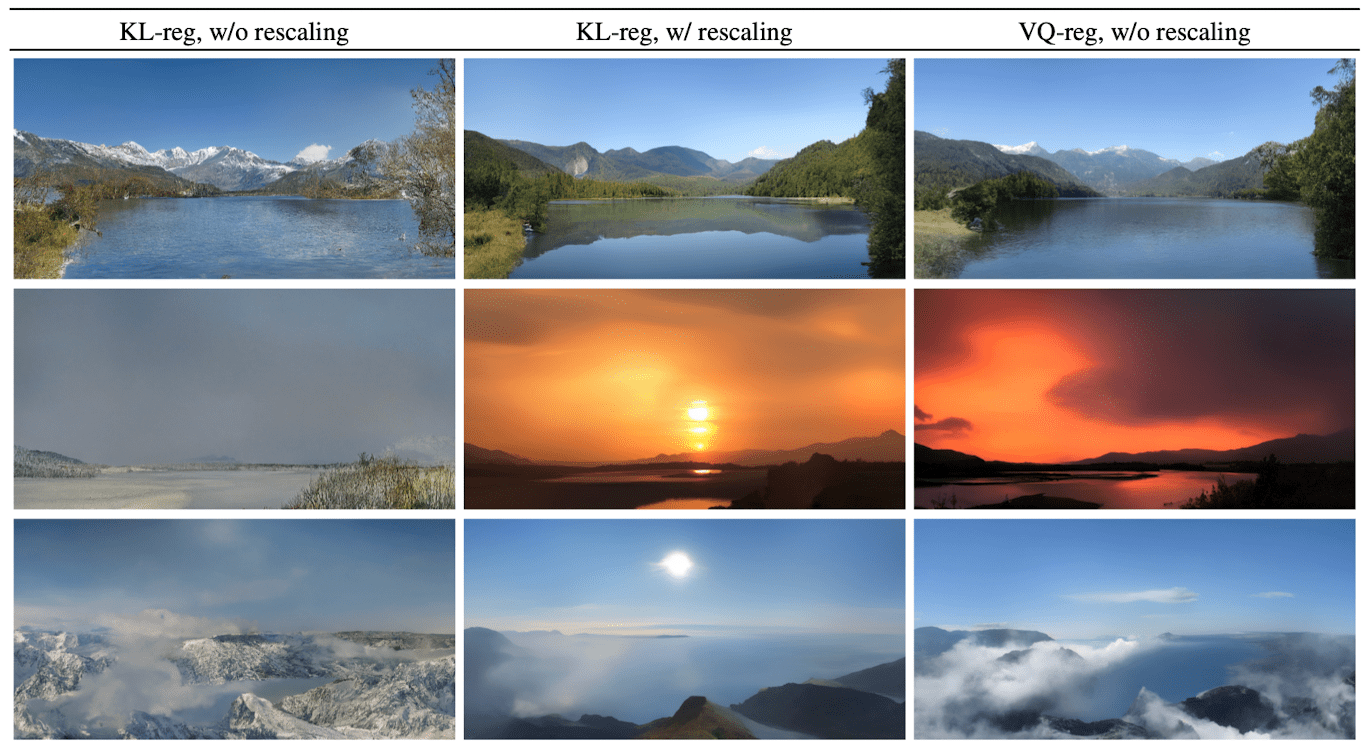
$\mathbf{Fig.}$ Effect of rescaling KL-reg latent space (Rombach et al. 2022)

\[\tag*{$\blacksquare$}\]

Then now the diffusion (forward) process and denoising (reverse) process can run on the low-dimensional latent vector $\mathbf{z}$. With fixed forward process, the denoising backbone is a conditional U-Net $\epsilon_{\theta} (\cdot, t, y)$, augmented with the cross-attention mechanism for more flexible conditioning image generation (e.g. class labels, text). The conditional information $y$ can be come from various modalities, therefore in order to fuse with UNet it required to be pre-processed via domain-specific encoder $\tau_\theta$ that projects $y$ to an intermediate representation $\tau_\theta (y) \in \mathbb{R}^{M \times d_{\tau}}$. Then it is mapped to the intermediate layers of the UNet by cross-attention component:

\[\begin{aligned} &\text{Attention}(\mathbf{Q}, \mathbf{K}, \mathbf{V}) = \text{softmax}\Big(\frac{\mathbf{Q}\mathbf{K}^\top}{\sqrt{d}}\Big) \cdot \mathbf{V} \\ &\text{with }\mathbf{Q} = \mathbf{W}^{(i)}_Q \cdot \varphi_i(\mathbf{z}_i),\; \mathbf{K} = \mathbf{W}^{(i)}_K \cdot \tau_\theta(y),\; \mathbf{V} = \mathbf{W}^{(i)}_V \cdot \tau_\theta(y) \\ \end{aligned}\]

where the learnable projection matrices \(\mathbf{W}^{(i)}_Q \in \mathbb{R}^{d \times d^i_\epsilon}\), \(\mathbf{W}^{(i)}_K, \mathbf{W}^{(i)}_V \in \mathbb{R}^{d \times d_\tau}\), a (flattened) intermediate representation of the UNet \(\varphi_i(\mathbf{z}_i) \in \mathbb{R}^{N \times d^i_\epsilon}\) and \(\tau_\theta(y) \in \mathbb{R}^{M \times d_\tau}\). Then the conditional LDM $\epsilon_\theta$ and domain specific encoder $\tau_\theta$ can be jointly optimized via

\[\begin{aligned} L_{\text{LDM}} = \mathbb{E}_{\mathcal{E}(\mathbf{x}), y, \epsilon \sim \mathcal{N}(\mathbf{0}, \mathbf{I}), t} \left[ \lVert \epsilon - \epsilon_{\theta} (\mathbf{z}_t, t, \tau_{\theta} (y)) \rVert_2^2 \right] \end{aligned}\]

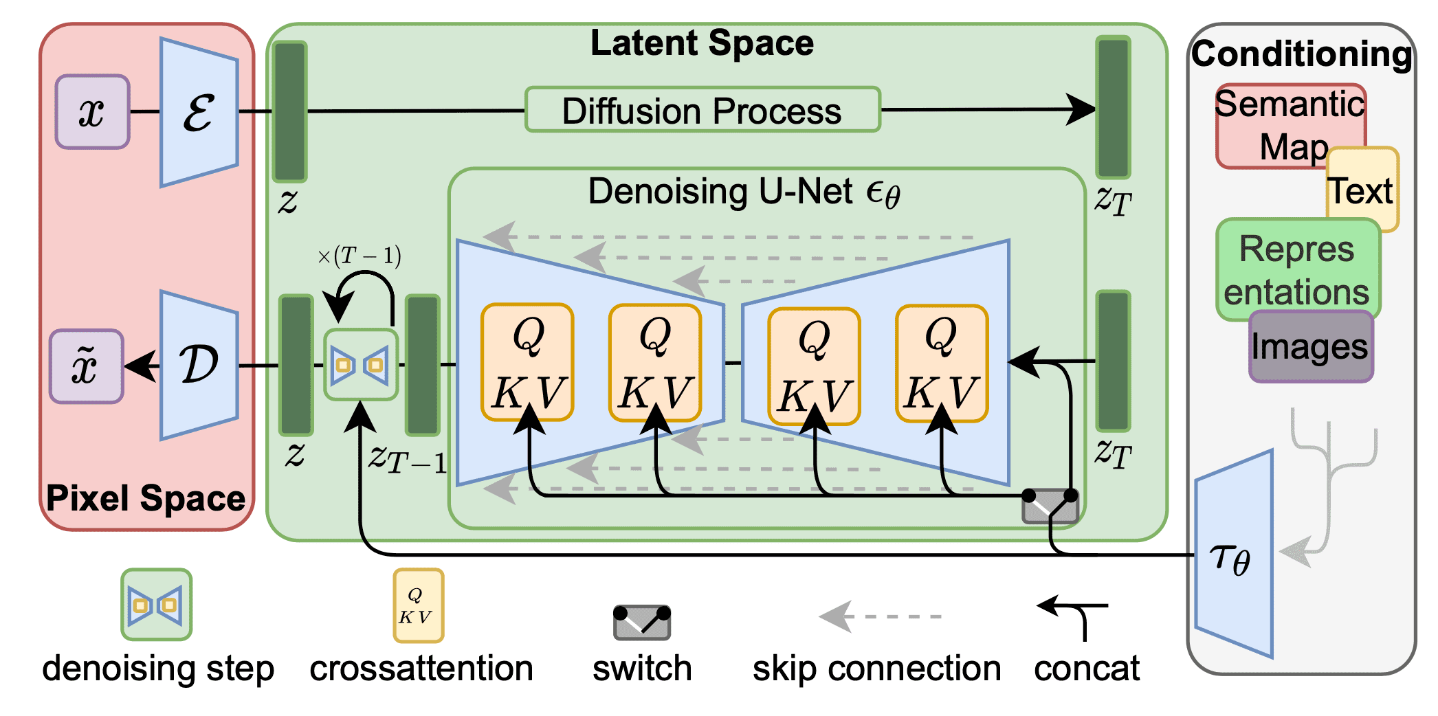
$\mathbf{Fig\ 2.}$ Latent Diffusion Model Architecture (Rombach et al. 2022)

Experiments

Perceptual Compression Tradeoffs

This section discusses the behavior of LDM with different downsampling factors \(f \in \{ 1, 2, 4, 8, 16, 32 \}\), abbreviated as LDM-$f$, where LDM-1 corresponds to pixel-based diffusion models.

• LDM-$1$ requires substantially longer training times
• LDM-$32$ compresses the data too much, thus limiting the overall sample quality.
• LDM-\(\{ 4 \sim 16 \}\) shows a good balance between efficiency and sample quality

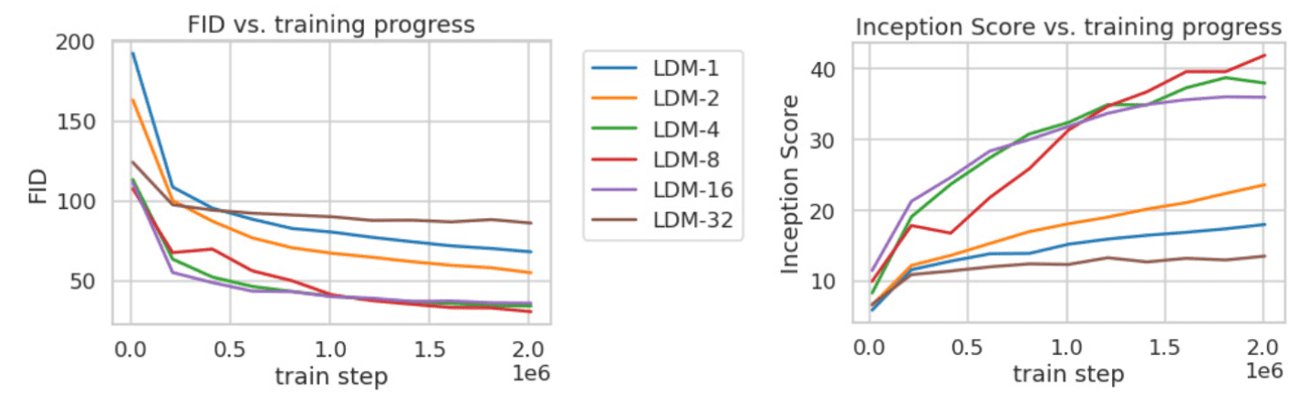
$\mathbf{Fig\ 3.}$ Image quality score comparisons with regard to $f$ (Rombach et al. 2022)

Unconditional Image Generation

LDMs successfully achieves the significant results on various unconditional image generation benchmarks, outperforming or getting close to the state-of-the-art results of the previous generative models including GANs. Also, LDMs outperform previous diffusion based approaches on all but the LSUN-Bedrooms dataset despite utilizing half its parameters and requiring 4-times less train resources.

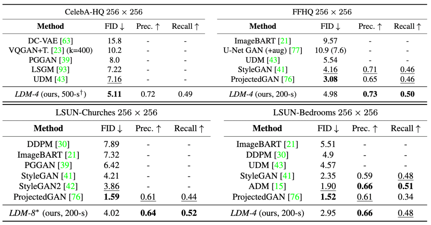
$\mathbf{Tab\ 1.}$ Evaluation metrics for unconditional image generation.
$N$-s refers to $N$ sampling steps with DDIM sampler, and $*$ refers to KL-reg. (Rombach et al. 2022)

$\mathbf{Fig\ 4.}$ Comparisons with other models (Rombach et al. 2022)

Conditional Image Generation

For text-to-image image modeling, the BERT-tokenizer with transformer-based $\tau_\theta$ is attached to the KL-regularized LDM, conditioned on language prompts on LAION-400M. And the resulting model shows the powerful results and generalizes well to complex, user-defined text prompts.

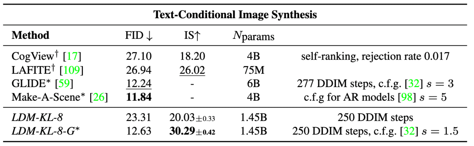
$\mathbf{Tab\ 2.}$ Comparisons with other models (Rombach et al. 2022)

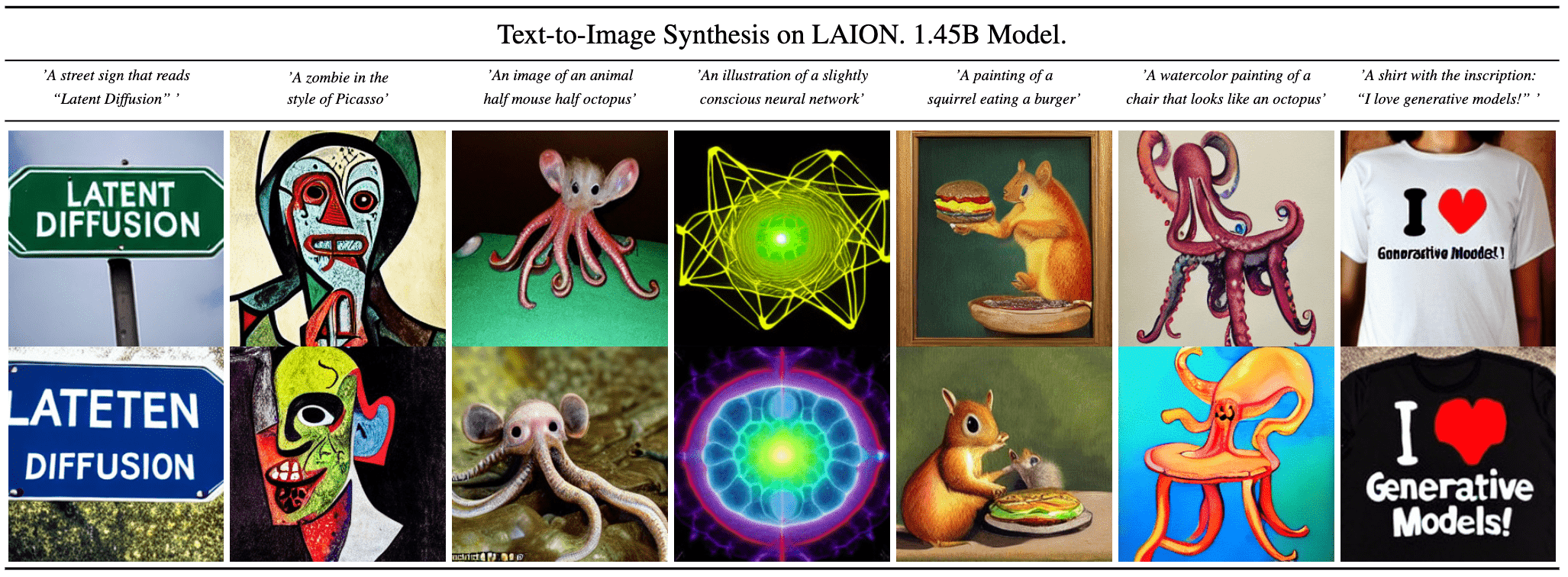
$\mathbf{Fig\ 5.}$ Comparisons with other models (Rombach et al. 2022)

Inpainting

In inpainting task, latent-based diffusion models sucessfully accelerate the training and inference time, while improving FID scores by a factor of at least $1.6\times$. Moreover, larger LDM with the scaled UNet that equips BigGAN residual block for up- and downsampling achieve the new state-of-the-art FID on image inpainting. (with fine-tuning for half an epoch to adjust the discrepancy between different resolutions)

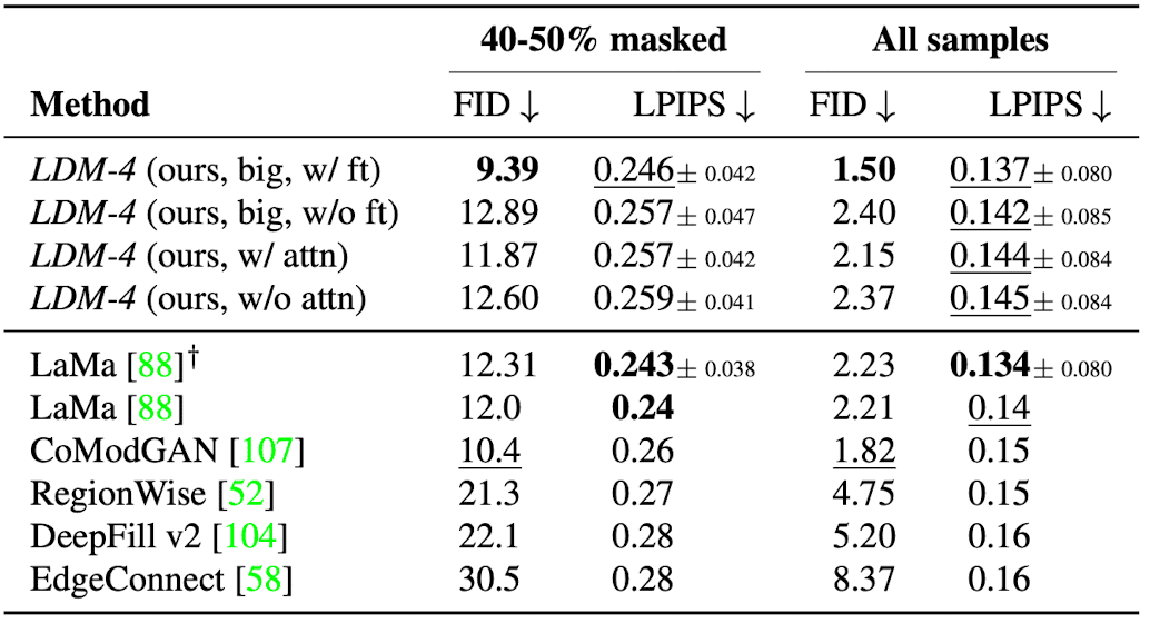
$\mathbf{Tab\ 3.}$ Comparison of inpainting performance on test images of Places dataset (Rombach et al. 2022)

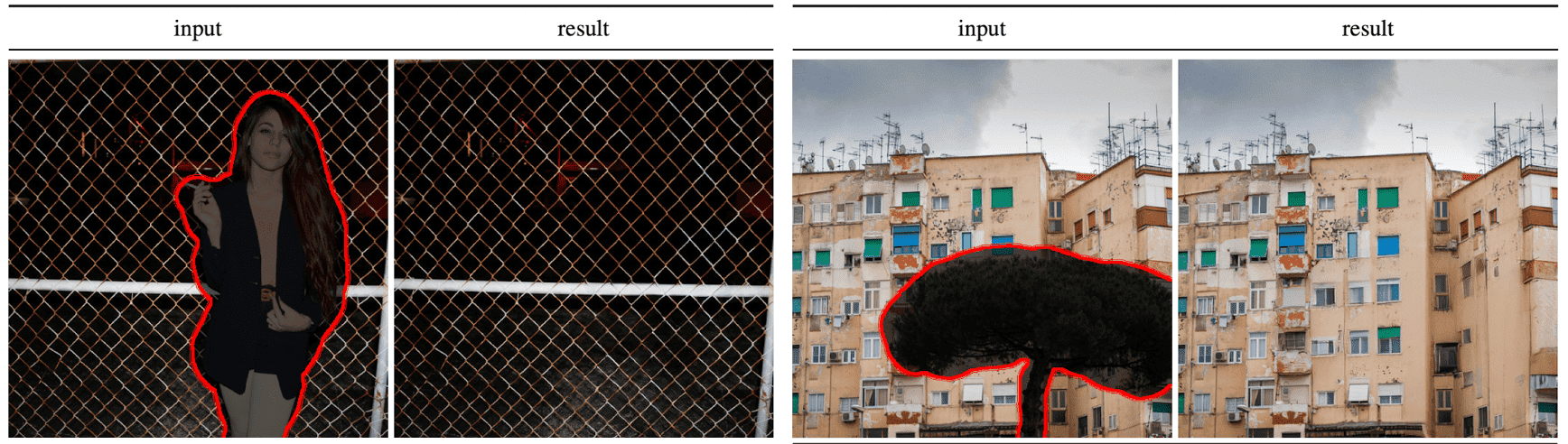
$\mathbf{Fig\ 6.}$ Qualitative results on object removal (Rombach et al. 2022)

Limitation

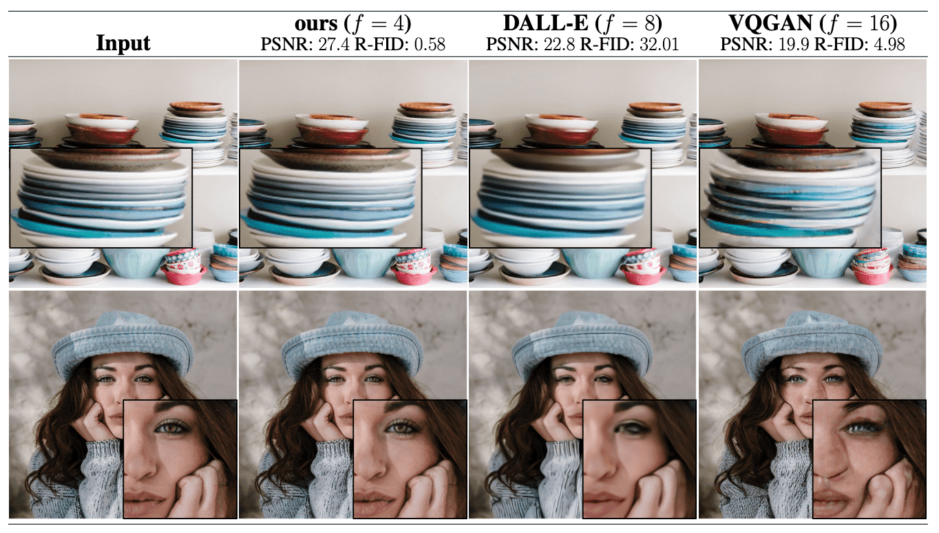
While latent diffusion models (LDMs) notably reduce computational burdens in contrast to pixel-based approaches, the sequential sampling process remains slower than that of Generative Adversarial Networks (GANs). Additionally, employing LDMs might raise concerns when demanding high precision: even though the image quality loss is marginal, their reconstruction ability might pose limitations for tasks that mandate precise accuracy in pixel space due to compression to the latent space.

Reference

[1] Rombach, Robin, et al. “High-Resolution Image Synthesis with Latent Diffusion Models.” CVPR 2022.