[Generative Model] Score Matching via SDEs

Introduction

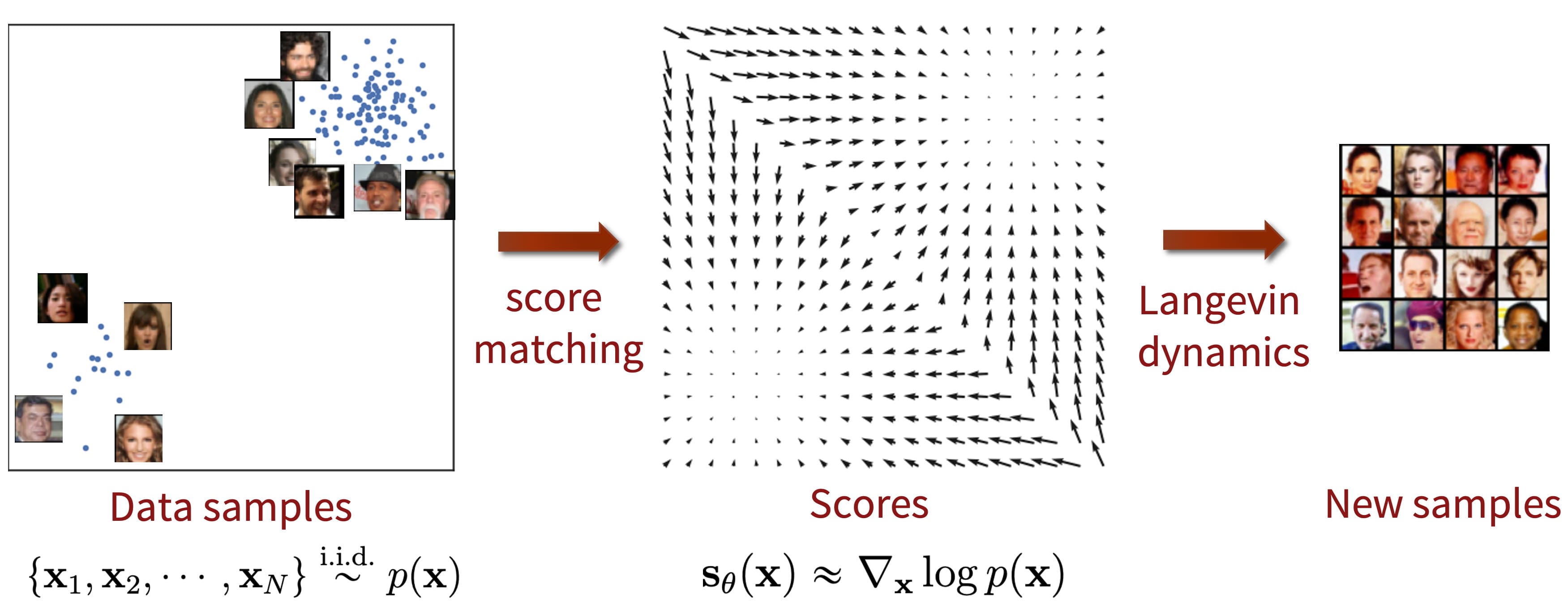
Score-based generative models have garnered significant attention due to the remarkable achievements of diffusion models. Notably, Song et al. ICLR 2021 introduces the stochastic differential equation (SDE) formulation of such score generative models, which serves as a generalized version of them. This formulation extends the timestep of forward/reverse processes to an infinite number of noise scales, enabling perturbed data distributions to evolve in accordance with an SDE as the noise intensity escalates.

$\mathbf{Fig\ 1.}$ Score-based generative model (source: Yang Song's blog)

SDE Formulation

A typical form of SDE, Itô SDE is given as follows:

\[\mathrm{d} \mathbf{x} = \mathbf{f}(\mathbf{x}, t) \mathrm{d} t + \mathbf{G}(\mathbf{x}, t) \mathrm{d} \mathbf{w}\]

where $t \in [0, T]$ resides in the continuous-time domain, $\mathbf{f}(\cdot, t): \mathbb{R}^d \to \mathbb{R}^d$ is the drift coefficient, $\mathbf{G}(\cdot, t): \mathbb{R}^d \to \mathbb{R}^{d \times d}$ is the diffusion coefficient, and $\mathbf{w}$ is the standard Wiener process. According to the theory of stochastic differential equations, it is mathematically known that the SDE has a unique strong solution if the coefficients are globally Lipschitz and satisfy a linear growth, i.e. for some constant $C$ and $D$, they satisfy

\[\begin{aligned} & \lVert \mathbf{f}(\mathbf{x}, t) \rVert + \lVert \mathbf{G}(\mathbf{x}, t) \rVert \leq C (1 + \lVert \mathbf{x} \rVert); \\ & \lVert \mathbf{f}(\mathbf{x}, t) - \mathbf{f}(\mathbf{y}, t) \rVert + \lVert \mathbf{G}(\mathbf{x}, t) - \mathbf{G}(\mathbf{y}, t) \rVert \leq D \lVert \mathbf{x} - \mathbf{y} \rVert; \\ \end{aligned}\]

Denote the probability density of the stochastic process \(\mathbf{x}_t\) by $p_t (\mathbf{x})$, where $0 \leq t \leq T$. Starting from samples of \(\mathbf{x}_T \sim p_T\), we obtain samples \(\mathbf{x}_0 \sim p_0\) via the reverse-time SDE, running backwards in time:

\[\mathrm{d} \mathbf{x} = [\mathbf{f}(\mathbf{x}, t) - \nabla \cdot [\mathbf{G}(\mathbf{x}, t) \mathbf{G}(\mathbf{x}, t)^\top] - \mathbf{G}(\mathbf{x}, t) \mathbf{G}(\mathbf{x}, t)^\top \nabla_{\mathbf{x}} \log p_t (\mathbf{x}) ] \mathrm{d}t + \mathbf{G}(\mathbf{x}, t) \mathrm{d} \bar{\mathbf{w}}\]

where $\bar{\mathbf{w}}$ is a standard Wiener process when time flows backwards from $T$ to $0$, and $\mathrm{d} t$ is an infinitesimal negative timestep. To estimate $\nabla_\mathbf{x} \log p_t (\mathbf{x})$, we can train time-dependent score-based model $\mathbf{s}_{\boldsymbol{\theta}} (\mathbf{x}, t)$:

\[\boldsymbol{\theta}^*=\underset{\boldsymbol{\theta}}{\arg \min} \; \mathbb{E}_{t \sim \mathcal{U}[0, T]} \left[\lambda_t \times \mathbb{E}_{\mathbf{x}_0 \sim p_0} \mathbb{E}_{\mathbf{x}_t \sim p_{0:t}}\left[\left\Vert\mathbf{s}_{\boldsymbol{\theta}}(\mathbf{x}_t, t)-\nabla_{\mathbf{x}_t} \log p_{0:t}(\mathbf{x}_t \mid \mathbf{x}_0)\right\Vert_2^2\right]\right] .\]

where $\mathcal{U}[0, T]$ denotes the uniform distribution over $[0, T]$, and $\lambda_t$ is a positive weighting function. As in DDPM, typically we set \(\lambda_t \propto 1/\mathbb{E}[\lVert \nabla_{\mathbf{x}_t} \log p_{0:t}(\mathbf{x}_t \mid \mathbf{x}_0) \rVert_2^2]\). And theoretically, we already know from the denosing score matching that this objective equivalently optimizes \(\mathbf{s}_{\boldsymbol{\theta}^*} (\mathbf{x}, t)\) that equals to $\nabla_{\mathbf{x}} \log p_{t} (\mathbf{x})$ almost all $\mathbf{x}$ and $t$.

Notice that to solve the optimization problem necessitates the transition kernel $p_{0:T}$. Although it simplifies to Gaussian distribution when the drift and diffusion coefficient of an SDE take the form of affine functions, it can be challenging to compute in general case. To circumvent this intractability, it is possible to employ sliced score matching:

\[\boldsymbol{\theta}^*=\underset{\boldsymbol{\theta}}{\arg \min} \; \mathbb{E}_{t \sim \mathcal{U}[0, T]} \left[\lambda_t \times \mathbb{E}_{\mathbf{x}_0} \mathbb{E}_{\mathbf{x}_t} \mathbb{E}_{\mathbf{v} \sim p_\mathbf{v}} \left[ \frac{1}{2} \left\Vert\mathbf{s}_{\boldsymbol{\theta}}(\mathbf{x}_t, t)\right\Vert_2^2 + \mathbf{v}^\top \mathbf{s}_{\boldsymbol{\theta}}(\mathbf{x}_t, t) \mathbf{v} \right]\right] .\]

Generation from the Reverse SDE

After training a time-dependent score-based model $\mathbf{s}_\boldsymbol{\theta}$, we can use it to construct the reverse-time SDE and then simulate it with numerical approaches to generate samples from $p_0$.

General-purpose Numerical SDE solvers

Numerical solvers provide approximate trajectories from SDEs. Many general-purpose numerical methods exist for solving SDEs, such as Euler-Maruyama and stochastic Runge-Kutta methods, which correspond to different discretizations of the stochastic dynamics. We can apply any of them to the reverse-time SDE for sample generation.

• Euler-Maruyama method
  It discretizes the SDE using finite time steps and small Gaussian noise. In the forward SDE $$ \mathrm{d} \mathbf{x}_t = \mathbf{f} (\mathbf{x}_t, t) \mathrm{d}t + \mathbf{G} (\mathbf{x}_t, t) \mathrm{d} \mathbf{w} $$ on some time interval $[0, T]$, it partitions the interval $[0, T]$ into $N$ equal subintervals of width $\Delta t = T / N$ iteratively approximate the true solution with the following Markov chain: $$ \mathbf{x}_{i + 1} = \mathbf{x}_i + \mathbf{f} (\mathbf{x}_i, t_i) \Delta t + \mathbf{G}(\mathbf{x}_i, t_i) \Delta \mathbf{w} \text{ where } \Delta \mathbf{w} = \mathbf{w}_{i + 1} - \mathbf{w}_i \sim \mathcal{N} (0, \Delta t \cdot \mathbf{I}) $$ Then, the Euler-Maruyama solver for our reverse SDE is given by $$ \begin{aligned} \mathbf{x}_{i} = & \; \mathbf{x}_{i+1} + [\mathbf{f}(\mathbf{x}_{i+1}, t_{i+1}) - \nabla \cdot [\mathbf{G}(\mathbf{x}_{i+1}, t_{i+1}) \mathbf{G}(\mathbf{x}_{i+1}, t_{i+1})^\top] - \mathbf{G}(\mathbf{x}_{i+1}, t_{i + 1}) \mathbf{G}(\mathbf{x}_{i+1}, t_{i + 1})^\top \mathbf{s}_\boldsymbol{\theta} (\mathbf{x}_{i+1}, t_{i + 1})] \Delta t \\ & + \mathbf{G}(\mathbf{x}_{i+1}, t) \sqrt{\vert \Delta t \vert} \; \mathbf{z}_i \text{ where } \mathbf{z}_i \sim \mathcal{N}(\mathbf{0}, \mathbf{I}) \end{aligned} $$ by approximating $\nabla_\mathbf{x} \log p_t (\mathbf{x}_t) \sim \mathbf{s}_\boldsymbol{\theta} (\mathbf{x}_, t)$, which flows $T \to 0$ with negative width $\Delta t < 0$.

Predictor-Corrector Samplers

Given that various numerical solvers exhibit distinct behaviors regarding the error of approximation, employing an off-the-shelf numerical solver for solving the ODE/SDE may yield various degrees of error. However, if we are specifically trying to solve the reverse diffusion equation, it is possible to use score-based MCMC approaches other than numerical ODE/SDE solvers to make the appropriate corrections.

Specifically, at each time step, the numerical SDE solver first gives an estimate of the sample at the next time step, playing the role of predictor. Then, the score-based MCMC approach corrects the marginal distribution of the estimated sample, playing the role of corrector.

$\mathbf{Fig\ 2.}$ Prediction and correction algorithm (Stanley Chan)

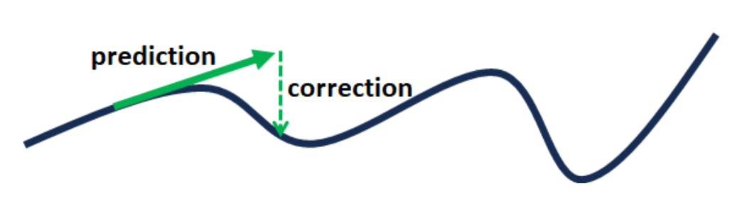
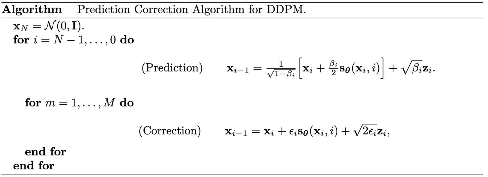
For instance, when using the reverse diffusion SDE solver as the predictor, and annealed Langevin dynamics (Euler-Maruyama method) as the corrector, DDPM alternates between two sampling rules:

\[\begin{alignat*}{2} \mathbf{x}_{i-1} & = \frac{1}{\sqrt{1 - \beta_i}} \left[ \mathbf{x}_i + \frac{\beta_i}{2} \nabla_{\mathbf{x}} \log p_i (\mathbf{x}_i) \right] + \sqrt{\beta_i} \mathbf{z}_i & \quad & \text{Prediction} \\ \mathbf{x}_{i-1} & = \mathbf{x}_i + \epsilon_i \nabla_{\mathbf{x}} \log p_i (\mathbf{x}_i) + \sqrt{2\epsilon_i} \mathbf{z}_i & \quad & \text{Correction} \end{alignat*}\]

$\mathbf{Fig\ 3.}$ Pseudocode for PC sampling (Stanley Chan)

Probability Flow ODE

Score-based models enable another numerical method for solving the reverse-time SDE.

$\color{red}{\mathbf{Theorem.}}$ Probability Flow ODE
Consider the SDE that possesses the following form: $$ \begin{gathered} \mathrm{d} \mathbf{x} = \mathbf{f}(\mathbf{x}, t) \mathrm{d}t + \mathbf{G} (\mathbf{x}, t) \mathrm{d} \mathbf{w} \\ \text{ where } \mathbf{f}(\cdot, t): \mathbb{R}^d \to \mathbb{R}^d, \mathbf{G}(\cdot, t): \mathbb{R}^d \to \mathbb{R}^{d \times d} \end{gathered} $$ Then, there exists a corresponding deterministic process whose trajectories share the same marginal probability densities $\{ p_t (\mathbf{x}) \}_{t=0}^T$ that satisfies an ODE, $$ \begin{gathered} \mathrm{d} \mathbf{x} = \left[ \tilde{\mathbf{f}} (\mathbf{x}, t) \right] \mathrm{d} t \\ \text{ where } \tilde{\mathbf{f}} (\mathbf{x}, t) := \mathbf{f}(\mathbf{x}, t) - \frac{1}{2} \nabla \cdot [\mathbf{G}(\mathbf{x}, t)\mathbf{G}(\mathbf{x}, t)^\top] - \frac{1}{2} \mathbf{G}(\mathbf{x}, t)\mathbf{G}(\mathbf{x}, t)^\top \nabla_\mathbf{x} \log p_t(\mathbf{x}). \end{gathered} $$ which is termed as probability flow ODE. This yields a deterministic iterative generation rule: $$ \mathbf{x}_i = \mathbf{x}_{i+1} - \mathbf{f}_{i+1}(\mathbf{x}_{i+1}) + \frac{1}{2}\mathbf{G}_{i+1}\mathbf{G}_{i+1}^\top \mathbf{s}_{\boldsymbol{\theta^*}} (\mathbf{x}_{i+1}, i+1) \quad i =0,1,\cdots, N-1, $$

$\mathbf{Proof.}$

The marginal probability density $p_t (\mathbf{x}(t))$ of Itô SDE can be obtained from the Fokker–Planck–Kolmogorov equation. It has mathematically proven that $p_t$ solves the following PDE:

\[\begin{aligned} \frac{\partial p_t(\mathbf{x})}{\partial t} & = -\sum_{i=1}^d \frac{\partial}{\partial x_i}[f_i(\mathbf{x}, t) p_t(\mathbf{x})] + \frac{1}{2}\sum_{i=1}^d\sum_{j=1}^d \frac{\partial^2}{\partial x_i \partial x_j}\left[\sum_{k=1}^d G_{ik}(\mathbf{x}, t) G_{jk}(\mathbf{x}, t) p_t(\mathbf{x})\right] \\ & = -\sum_{i=1}^d \frac{\partial}{\partial x_i}[f_i(\mathbf{x}, t) p_t(\mathbf{x})] + \frac{1}{2}\sum_{i=1}^d \frac{\partial}{\partial x_i} \left[ \sum_{j=1}^d \frac{\partial}{\partial x_j}\left[\sum_{k=1}^d G_{ik}(\mathbf{x}, t) G_{jk}(\mathbf{x}, t) p_t(\mathbf{x})\right]\right] \end{aligned}\]

Observe that the inner part of RHS is rewritten by chain rule:

\[\begin{aligned} &\sum_{j=1}^d \frac{\partial}{\partial x_j}\left[\sum_{k=1}^d G_{ik}(\mathbf{x}, t) G_{jk}(\mathbf{x}, t) p_t(\mathbf{x})\right]\\ =& \sum_{j=1}^d \frac{\partial}{\partial x_j} \left[ \sum_{k=1}^d G_{ik}(\mathbf{x}, t) G_{jk}(\mathbf{x}, t) \right] p_t(\mathbf{x}) + \sum_{j=1}^d \sum_{k=1}^d G_{ik}(\mathbf{x}, t)G_{jk}(\mathbf{x}, t) p_t(\mathbf{x}) \frac{\partial}{\partial x_j} \log p_t(\mathbf{x})\\ =& \; p_t(\mathbf{x}) \nabla \cdot [\mathbf{G}(\mathbf{x}, t)\mathbf{G}(\mathbf{x}, t)^\top] + p_t(\mathbf{x}) \mathbf{G}(\mathbf{x}, t)\mathbf{G}(\mathbf{x}, t)^\top \nabla_\mathbf{x} \log p_t(\mathbf{x}) \end{aligned}\]

By concatenating with the LHS:

\[\begin{aligned} \frac{\partial p_t(\mathbf{x})}{\partial t} &= -\sum_{i=1}^d \frac{\partial}{\partial x_i}[f_i(\mathbf{x}, t) p_t(\mathbf{x})] \\ &\quad + \frac{1}{2}\sum_{i=1}^d \frac{\partial}{\partial x_i} \Big[ p_t(\mathbf{x}) \nabla \cdot [\mathbf{G}(\mathbf{x}, t)\mathbf{G}(\mathbf{x}, t)^\top] + p_t(\mathbf{x}) \mathbf{G}(\mathbf{x}, t)\mathbf{G}(\mathbf{x}, t)^\top \nabla_\mathbf{x} \log p_t(\mathbf{x}) \Big] \\ &= -\sum_{i=1}^d \frac{\partial}{\partial x_i}\Big\{ f_i(\mathbf{x}, t)p_t(\mathbf{x}) \\ &\quad - \frac{1}{2} \Big[ \nabla \cdot [\mathbf{G}(\mathbf{x}, t)\mathbf{G}(\mathbf{x}, t)^\top] + \mathbf{G}(\mathbf{x}, t)\mathbf{G}(\mathbf{x}, t)^\top \nabla_\mathbf{x} \log p_t(\mathbf{x}) \Big] p_t(\mathbf{x}) \Big\} \\ &= -\sum_{i=1}^d \frac{\partial}{\partial x_i} [\tilde{f}_i(\mathbf{x}, t)p_t(\mathbf{x})] \end{aligned}\]

where we denote

\[\tilde{\mathbf{f}}(\mathbf{x}, t) := \mathbf{f}(\mathbf{x}, t) - \frac{1}{2} \nabla \cdot [\mathbf{G}(\mathbf{x}, t)\mathbf{G}(\mathbf{x}, t)^\top] - \frac{1}{2} \mathbf{G}(\mathbf{x}, t)\mathbf{G}(\mathbf{x}, t)^\top \nabla_\mathbf{x} \log p_t(\mathbf{x}).\]

Note that the final equation equals to Fokker–Planck–Kolmogorov equation of the following Itô SDE:

\[\mathrm{d} \mathbf{x} = \tilde{\mathbf{f}} (\mathbf{x}, t) \; \mathrm{d}t\] \[\tag*{$\blacksquare$}\]

Using the estimated probability flow ODE with the score network $\mathbf{s}_{\boldsymbol{\theta}} (\mathbf{x}, t)$:

\[\mathrm{d} \mathbf{x} = \underbrace{\left\{\mathbf{f}(\mathbf{x}, t) - \frac{1}{2} \nabla \cdot [\mathbf{G}(\mathbf{x}, t)\mathbf{G}(\mathbf{x}, t)^\top] - \frac{1}{2} \mathbf{G}(\mathbf{x}, t)\mathbf{G}(\mathbf{x}, t)^\top \mathbf{s}_\boldsymbol{\theta}(\mathbf{x}, t)\right\}}_{=: \tilde{\mathbf{f}}_\boldsymbol{\theta} (\mathbf{x}, t)} \; \mathrm{d} t\]

and the instantaneous change of variables theorem (proved in Neural ODE paper) when $g (\mathbf{x}(t), t) = \frac{\mathrm{d} \mathbf{x}}{\mathrm{d} t}$ is uniformly Lipschitz continuous in $\mathbf{x}$ and $t$:

\[\frac{\partial \log p(\mathbf{x} (t))}{\partial t} = - \nabla_{\mathbf{x}(t)} \cdot g (\mathbf{x}(t), t)\]

we can compute that log-likelihood of data distribution $p_0 (\mathbf{x})$ with

\[\begin{gathered} \log p_T(\mathbf{x}(T)) - \log p_0(\mathbf{x}(0)) = \int_0^T \frac{\partial \log p(\mathbf{x} (t))}{\partial t} \mathrm{d} t \\ \Leftrightarrow \log p_0(\mathbf{x}(0)) = \log p_T(\mathbf{x}(T)) + \int_0^T \nabla \cdot \tilde{\mathbf{f}}_\boldsymbol{\theta}(\mathbf{x}(t), t) \mathrm{d} t \end{gathered}\]

where $\mathbf{x}(t)$ can be obtained by solving the probability flow ODE.

Discretization to NCSN and DDPM

Indeed, the SDE formulation of score matching serves as the generalized framework of score-based generative models such as NCSN and DDPM. By discretizing the time domain of the Variance Exploding (VE) SDE and Variance Preserving (VP) SDE, our formulation reduces to NCSN and DDPM, respectively.

Variance Exploding (VE) SDE

Recall that NCSN perturbs the data with various levels of noise \(\{ \sigma_i \}_{i=1}^N\) and perturbation kernel $p_\sigma (\tilde{\mathbf{x}} \vert \mathbf{x}) = \mathcal{N}(\tilde{\mathbf{x}} \vert \mathbf{x}, \sigma^2 \mathbf{I})$ to prevent the data from being confined to a low dimensional manifold. Then, each perturbation kernel $p_{\sigma_i} (\mathbf{x} \vert \mathbf{x}_0)$ can be expressed by the following Markov chain:

\[\mathbf{x}_{i} = \mathbf{x}_{i-1} + (\sigma_i^2 - \sigma_{i-1}^2) \mathbf{z}_{i-1} \quad \text{ where } \mathbf{z}_{i-1} \sim \mathcal{N} (\mathbf{0}, \mathbf{I}) \text{ and } i = 1, \cdots, N\]

with the notation \(\mathbf{x}_0 \sim p_{\mathrm{data}}\) and $\sigma_0 = 0$. In the limit case $N \to \infty$, the above Markov chain can be written as continuous stochastic process $\mathbf{x} (t)$ with $t \in [0, 1]$ with $\sigma(t)$, $\mathbf{z}(t)$ by letting $t = \frac{i}{N}$, where $\mathbf{x}(\frac{i}{N}) = \mathbf{x}_i$, $\sigma(\frac{i}{N}) = \sigma_i$, and $\mathbf{z}(\frac{i}{N}) = \mathbf{z}_i$. With $\Delta t = \frac{1}{N}$ and \(t = \{ 0, \frac{1}{N}, \cdots, \frac{N-1}{N} \}\), the above equation is rewritten as follows:

\[\mathbf{x} (t + \Delta t) = \mathbf{x}(t) + \sqrt{\sigma^2 (t + \Delta t) - \sigma^2 (t)} \; \mathbf{z} (t) \approx \mathbf{x}(t) + \sqrt{\frac{\mathrm{d} \sigma^2 (t)}{\mathrm{d} t} \Delta t} \; \mathbf{z}_t\]

where the approximation holds when $\Delta t \ll 1$. Since Wiener process has Gaussian increment, when $\Delta t \to 0$, it turns out to be

\[\mathrm{d} \mathbf{x} = \sqrt{\frac{\mathrm{d} \sigma^2 (t)}{\mathrm{d} t}} \mathrm{d} \mathbf{w}\]

which is termed variance exploding (VE) SDE. This implies the following reverse equation of NSCN:

\[\mathrm{d} \mathbf{x} = - \left( \frac{\mathrm{d} [\sigma(t)^2]}{\mathrm{d} t} \nabla_{\mathbf{x}} \log p_t (\mathbf{x}(t)) \right) \mathrm{d}t + \sqrt{\frac{\mathrm{d} [\sigma(t)^2]}{\mathrm{d}t}} \mathrm{d} \bar{\mathbf{w}}\]

For brevity, define $\alpha(t) = \tfrac{\mathrm{d} [\sigma(t)^2]}{\mathrm{d} t}$. Then, by the discretization with \(\mathbf{x}(t + \Delta t) = \mathbf{x}_{i}\), \(\mathbf{x}(t) = \mathbf{x}_{i-1}\), and \(\alpha (t) \Delta t = \alpha_i\), considering $\mathrm{d} \bar{\mathbf{w}} = \mathbf{w} (t - \Delta t) - \mathbf{w}(t) = - \mathbf{z}(t)$, we obtain

\[\begin{alignat}{2} & \quad & \mathbf{x}(t + \Delta t) - \mathbf{x}(t) & = - \Big( \alpha(t) \nabla_{\mathbf{x}} \log p_t(\mathbf{x})\Big) \Delta t - \sqrt{\alpha(t)\Delta t} \; \mathbf{z}(t) \\ & \Leftrightarrow \quad & \mathbf{x}(t) & = \mathbf{x}(t+\Delta t) + \alpha(t)\Delta t \nabla_{\mathbf{x}} \log p_t(\mathbf{x}) + \sqrt{\alpha(t)\Delta t} \; \mathbf{z}(t) \\ & \Leftrightarrow \quad & \mathbf{x}_{i-1} &= \mathbf{x}_i + \alpha_i \nabla_{\mathbf{x}} \log p_i(\mathbf{x}_i) + \sqrt{\alpha_i} \; \mathbf{z}_i \\ & \Leftrightarrow \quad & \mathbf{x}_{i-1} &= \mathbf{x}_i + (\sigma_i^2-\sigma_{i-1}^2) \nabla_{\mathbf{x}} \log p_i(\mathbf{x}_i) + \sqrt{(\sigma_i^2-\sigma_{i-1}^2)} \; \mathbf{z}_i, \end{alignat}\]

that is identical to the original annealed Langevin dynamics sampling of NCSN.

Variance Preserving (VP) SDE

Recall that DDPM maps the data distribution to the noise distribution by gradually adding Gaussian noise to the data based on variance schedule $\beta_1, \cdots, \beta_N$ with the perturbation kernel \(\{ p_{\beta_i} (\mathbf{x} \vert \mathbf{x}_0) \}_{i=1}^N\)

\[\begin{gathered} p_{\beta_i} (\mathbf{x}_i \vert \mathbf{x}_{i-1}) = \mathcal{N} (\sqrt{1 - \beta_i} \mathbf{x}_{i-1}, \beta_i \mathbf{I}) \\ \Leftrightarrow \mathbf{x}_i = \sqrt{1 - \beta_i} \mathbf{x}_{i-1} + \sqrt{\beta_i} \mathbf{z}_{i-1} \text{ where } \mathbf{z}_{i-1} \sim \mathcal{N} (\mathbf{0}, \mathbf{I}) \end{gathered}\]

In the limit case $N \to \infty$, the above Markov chain can be written as continuous SDE. To obtain the limit, define an auxiliary set of noise schedules \(\{ \bar\beta_i = N \beta_i \}_{i=1}^N\). By letting $\beta (\frac{i}{N}) = \bar\beta_i$, $\mathbf{x}(\frac{i}{N}) = \mathbf{x}_i$, and $\mathbf{z} (\frac{i}{N}) = \mathbf{z}_i$ with $\Delta t = \frac{1}{N}$ and \(t = \{ 0, \frac{1}{N}, \cdots, \frac{N-1}{N} \}\), the above equation is rewritten as follows:

\[\begin{aligned} \mathbf{x}(t+\Delta t) & =\sqrt{1-\beta(t+\Delta t) \Delta t} \; \mathbf{x}(t)+\sqrt{\beta(t+\Delta t) \Delta t} \; \mathbf{z}(t) \\ & \approx \mathbf{x}(t)-\frac{1}{2} \beta(t+\Delta t) \Delta t \; \mathbf{x}(t)+\sqrt{\beta(t+\Delta t) \Delta t} \; \mathbf{z}(t) \\ & \approx \mathbf{x}(t)-\frac{1}{2} \beta(t) \Delta t \; \mathbf{x}(t) + \sqrt{\beta(t) \Delta t} \; \mathbf{z}(t) \end{aligned}\]

where the approximation holds when $\Delta t \ll 1$. Since Wiener process has Gaussian increment, when $\Delta t \to 0$, it turns out to be

\[\mathrm{d} \mathbf{x} = - \frac{1}{2} \beta (t) \mathbf{x} \; \mathrm{d} t + \sqrt{\beta (t)} \; \mathrm{d}\mathbf{w}.\]

Song and Ermon called this SDE an variance preserving (VP) SDE. Then, the reverse sampling equation of DDPM can be written as an SDE via

\[\mathrm{d} \mathbf{x} = -\beta(t) \left[ \frac{\mathbf{x}}{2} + \nabla_{\mathbf{x}} \; p_t (\mathbf{x}) \right] \mathrm{d}t + \sqrt{\beta(t)} \mathrm{d} \bar{\mathbf{w}}\]

Again, the discretized iterative update rule can be obtained by considering $\mathrm{d} \mathbf{x} = \mathbf{x}(t) - \mathbf{x}(t - \Delta t)$ and $\mathrm{d} \bar{\mathbf{w}} = \mathbf{w} (t - \Delta t) - \mathbf{w}(t) = - \mathbf{z}(t)$:

\[\mathbf{x}(t - \Delta t) = \mathbf{x}(t) + \beta (t) \Delta t \left[ \frac{\mathbf{x}(t)}{2} + \nabla_{\mathbf{x}} \log p_t (\mathbf{x}(t)) \right] + \sqrt{\beta(t) \Delta t} \; \mathbf{z}(t)\]

Assuming that $\beta (t) \Delta t \ll 1$, it can be further rewritten as

\[\begin{aligned} \mathbf{x}(t-\Delta t) &= \mathbf{x}(t)\left[1 + \frac{\beta(t)\Delta t}{2} \right] + \beta(t)\Delta t \nabla_{\mathbf{x}} \log p_t(\mathbf{x}(t)) + \sqrt{\beta(t)\Delta t} \mathbf{z}(t) \\ &\approx \mathbf{x}(t)\left[1 + \frac{\beta(t)\Delta t}{2} \right] + \beta(t)\Delta t \nabla_{\mathbf{x}} \log p_t(\mathbf{x}(t)) + \color{blue}{ \tfrac{(\beta(t)\Delta t)^2}{2} \nabla_{\mathbf{x}} \log p_t(\mathbf{x}(t))} + \sqrt{\beta(t)\Delta t} \mathbf{z}(t) \\ &= \left[1 + \frac{\beta(t)\Delta t}{2} \right]\left( \mathbf{x}(t) + \beta(t)\Delta t \nabla_{\mathbf{x}} \log p_t(\mathbf{x}(t)) \right) + \sqrt{\beta(t)\Delta t} \mathbf{z}(t). \end{aligned}\]

The discretization with $\mathbf{x}(t-\Delta t) = \mathbf{x}_{i-1}$, $\mathbf{x}(t) = \mathbf{x}_i$, and $\beta (t) \Delta t = \beta_i$ provides the following sampling rule:

\[\begin{align} \mathbf{x}_{i-1} &= (1+\frac{\beta_i}{2})\left[ \mathbf{x}_i + \frac{\beta_i}{2} \nabla_{\mathbf{x}} \log p_i(\mathbf{x}_i) \right] + \sqrt{\beta_i} \mathbf{z}_i \\ &\approx \frac{1}{\sqrt{1-\beta_i}} \left[ \mathbf{x}_i + \frac{\beta_i}{2} \nabla_{\mathbf{x}} \log p_i(\mathbf{x}_i) \right] + \sqrt{\beta_i} \mathbf{z}_i \end{align}\]

References

[1] Song et al., “Score-Based Generative Modeling through Stochastic Differential Equations” ICLR 2021 Oral..
[2] Chan et al., “Tutorial on Diffusion Models for Imaging and Vision”, arXiv:202403.18103
[3] Wikipedia, Euler-Maruyama method
[4] Chen et al., “Neural Ordinary Differential Equations”, NeurIPS 2018
[5] Pierzchlewicz, Paweł A. (Jul 2022). Langevin Monte Carlo: Sampling using Langevin Dynamics. Perceptron.blog.
[6] Särkkä, Simo and Solin, Arno, “Applied Stochastic Differential Equations”, Cambridge University Press, 2019.