
[Generative Model] Guided Diffusion
Introduction
Despite GANs holding the state-of-the-art in most image synthesis benchmarks, their limitations, such as a lack of sample diversity, pose challenges for scalability and application to new domains. Consequently, efforts have been directed towards achieving GAN-like sample quality with likelihood-based models. While these models encompass more diversity and are generally more manageable to scale and train than GANs, they still lag behind in terms of sample quality. Additionally, excluding VAEs, sampling from these models is slower than GANs.
Among likelihood-based models, diffusion models have emerged as a noteworthy generative model, showcasing the production of high-quality images while maintaining advantageous properties such as distribution coverage, a stationary training objective, and scalability. However, diffusion models are inferior to GANs on challenging datasets, including ImageNet.
To improve the sampling quality of diffusion models, Dhariwal & Nichol et al. NeurIPS 2021 firstly proposed the extra technique of guidance of diffusion generation termed classifier guidance with the following basic idea:
If we have additional information about the data, such as class labels for images, can we utilize this information to improve the quality of generation?
In this post, we explore diverse guidance techniques for diffusion models, a set of strategies that have accelerated the practical deployment of diffusion in real-world applications.
Classifier Guidance
First, we can exploit additional information about the data with conditional reverse noising process:
\[\begin{aligned} p_{\theta, \phi} (\mathbf{x}_t \vert \mathbf{x}_{t + 1}, y) & = \frac{p_{\theta, \phi} (\mathbf{x}_t, \mathbf{x}_{t+1}, y)}{p_{\theta, \phi} (\mathbf{x}_{t+1}, y)} \\ & = \frac{p_{\theta, \phi} (\mathbf{x}_t \vert \mathbf{x}_{t+1}) p_{\theta, \phi}(y \vert \mathbf{x}_t, \mathbf{x}_{t+1})}{p_{\theta, \phi} (y \vert \mathbf{x}_{t+1})} \\ & = \frac{p_{\theta, \phi} (\mathbf{x}_t \vert \mathbf{x}_{t+1}) p_{\theta, \phi}(y \vert \mathbf{x}_t)}{p_{\theta, \phi} (y \vert \mathbf{x}_{t+1})} & \because \text{Markov property} \\ & = \frac{p_{\theta} (\mathbf{x}_t \vert \mathbf{x}_{t+1}) p_{\phi}(y \vert \mathbf{x}_t)}{p_{\phi} (y \vert \mathbf{x}_{t+1})} \\ & = \frac{p_{\theta} (\mathbf{x}_t \vert \mathbf{x}_{t+1}) p_{\phi}(y \vert \mathbf{x}_t)}{Z} \end{aligned}\]where $Z$ is a normalizing constant. Although it is intractable to sample from the distribution exactly, we can approximate it as a perturbed Gaussian distribution.
$\mathbf{Proof.}$
Recall that our usual diffusion model predicts the previous timestep \(\mathbf{x}_t\) from timestep \(\mathbf{x}_{t+1}\) using a Gaussian distribution:
\[\begin{aligned} p_{\theta} (\mathbf{x}_t \vert \mathbf{x}_{t+1}) & = \mathcal{N} (\boldsymbol{\mu}_\theta(\mathbf{x}_t, t), \boldsymbol{\Sigma}_\theta(\mathbf{x}_t, t)) \\ \log p_{\theta} (\mathbf{x}_t \vert \mathbf{x}_{t+1}) & = - \frac{1}{2} (\mathbf{x}_t - \boldsymbol{\mu}_\theta(\mathbf{x}_t, t))^\top \boldsymbol{\Sigma}_\theta^{-1} (\mathbf{x}_t, t) (\mathbf{x}_t - \boldsymbol{\mu}_\theta(\mathbf{x}_t, t)) + C_1 \\ \end{aligned}\]We can assume that \(\log p_{\theta} (\mathbf{x}_t \vert \mathbf{x}_{t+1})\) has low curvature compared to \(\boldsymbol{\Sigma}_\theta^{-1}\). It is reasonable in the limit of infinite diffusion steps, where \(\lVert \boldsymbol{\Sigma}_\theta (\mathbf{x}_t, t) \rVert \to 0\). And in general, we set \(\boldsymbol{\Sigma}_\theta (\mathbf{x}_t, t) = \sigma_t^2 \mathbf{I}\) where $\sigma_t^2 \propto \beta_t$ and very small $\beta_t$. With this assumption, we can use a Taylor expansion around \(\mathbf{x}_t = \boldsymbol{\mu}_\theta(\mathbf{x}_t, t)\) as
\[\begin{aligned} \log p_{\theta} (\mathbf{x}_t \vert \mathbf{x}_{t+1}) & \approx \log p_{\theta} (\mathbf{x}_t \vert \mathbf{x}_{t+1}) \vert_{\mathbf{x}_t = \boldsymbol{\mu}_\theta(\mathbf{x}_t, t)} + (\mathbf{x}_t = \boldsymbol{\mu}_\theta(\mathbf{x}_t, t)) \nabla_{\mathbf{x}_t} \log p_{\theta} (\mathbf{x}_t \vert \mathbf{x}_{t+1}) \vert_{\mathbf{x}_t = \boldsymbol{\mu}_\theta(\mathbf{x}_t, t)} \\ & = (\mathbf{x}_t - \boldsymbol{\mu}_\theta(\mathbf{x}_t, t)) \mathbf{g} + C_2 \end{aligned}\]Finally, we obtain
\[\begin{aligned} \log \left(p_\theta\left(\mathbf{x}_t \mid \mathbf{x}_{t+1} \right) p_\phi\left(y \mid \mathbf{x}_t \right)\right) & \approx -\frac{1}{2}\left(\mathbf{x}_t -\boldsymbol{\mu}_\theta \right)^\top \boldsymbol{\Sigma}_\theta ^{-1}\left(\mathbf{x}_t -\boldsymbol{\mu}_\theta \right)+\left(\mathbf{x}_t -\boldsymbol{\mu}_\theta \right) \mathbf{g} + C_2 \\ & = -\frac{1}{2}\left(\mathbf{x}_t -\boldsymbol{\mu}_\theta -\boldsymbol{\Sigma}_\theta \mathbf{g} \right)^\top \boldsymbol{\Sigma}_\theta^{-1} \left(\mathbf{x}_t -\boldsymbol{\mu}_\theta -\boldsymbol{\Sigma}_\theta \mathbf{g} \right)+\frac{1}{2} \mathbf{g}^\top \boldsymbol{\Sigma}_\theta \mathbf{g} + C_2 \\ & = -\frac{1}{2}\left(\mathbf{x}_t - \boldsymbol{\mu}_\theta -\boldsymbol{\Sigma}_\theta \mathbf{g} \right)^\top \boldsymbol{\Sigma}_\theta^{-1}\left(\mathbf{x}_t -\boldsymbol{\mu}_\theta - \boldsymbol{\Sigma}_\theta \mathbf{g} \right)+C_3 \\ & = \log p(\mathbf{z}) + C \quad \mathbf{z} \sim \mathcal{N}(\boldsymbol{\mu}_\theta + \boldsymbol{\Sigma}_\theta \mathbf{g}, \boldsymbol{\Sigma}_\theta ) \end{aligned}\]We have thus found that the conditional reverse process can be approximated by a Gaussian similar to the unconditional reverse process, but with its mean shifted by \(\boldsymbol{\Sigma}_\theta \mathbf{g}\).
\[\tag*{$\blacksquare$}\]Note that the above process is only applicable to stochastic sampler (DDPM), but not to deterministic sampler (DDIM). To improve a general diffusion generator, Dhariwal & Nichol et al. 2021 exploit a trained classifier \(p_{\phi} (y \vert \mathbf{x}_t)\) on noisy images \(\mathbf{x}_t\), and then guide the diffusion sampling process towards the class label $y$, with its gradients \(\nabla_{\mathbf{x}_t} \log p_{\phi} (y \vert \mathbf{x}_t)\). Recall that the score network of diffusion approximates \(\nabla_{\mathbf{x}_t} \log q(\mathbf{x}_t)\) by noise prediction: \(\mathbf{s}_{\theta} (\mathbf{x}_t, t) = - \frac{\boldsymbol{\epsilon}_{\theta} (\mathbf{x}_t, t)}{\sqrt{1 - \bar{\alpha}_t}}\). Then we have
\[\begin{aligned} \nabla_{\mathbf{x}_t} \log q(\mathbf{x}_t \vert y) \propto \nabla_{\mathbf{x}_t} \log q(\mathbf{x}_t, y) &= \nabla_{\mathbf{x}_t} \log q(\mathbf{x}_t) + \nabla_{\mathbf{x}_t} \log q(y \vert \mathbf{x}_t) \\ &\approx - \frac{1}{\sqrt{1 - \bar{\alpha}_t}} \boldsymbol{\epsilon}_\theta(\mathbf{x}_t, t) + \nabla_{\mathbf{x}_t} \log q(y \vert \mathbf{x}_t) \\ &= - \frac{1}{\sqrt{1 - \bar{\alpha}_t}} \left[\boldsymbol{\epsilon}_\theta(\mathbf{x}_t, t) - \sqrt{1 - \bar{\alpha}_t} \nabla_{\mathbf{x}_t} \log q(y \vert \mathbf{x}_t)\right] \end{aligned}\]To compute \(\nabla_{\mathbf{x}_t} \log q(y \vert \mathbf{x}_t)\), we will approximate it by \(\nabla_{\mathbf{x}_t} \log p_{\phi}(y \vert \mathbf{x}_t)\). Hence, we can define a new noise predictor \(\hat{\boldsymbol{\epsilon}}_{\theta} (\mathbf{x}_t, t)\) to correspond to the score of the joint distribution:
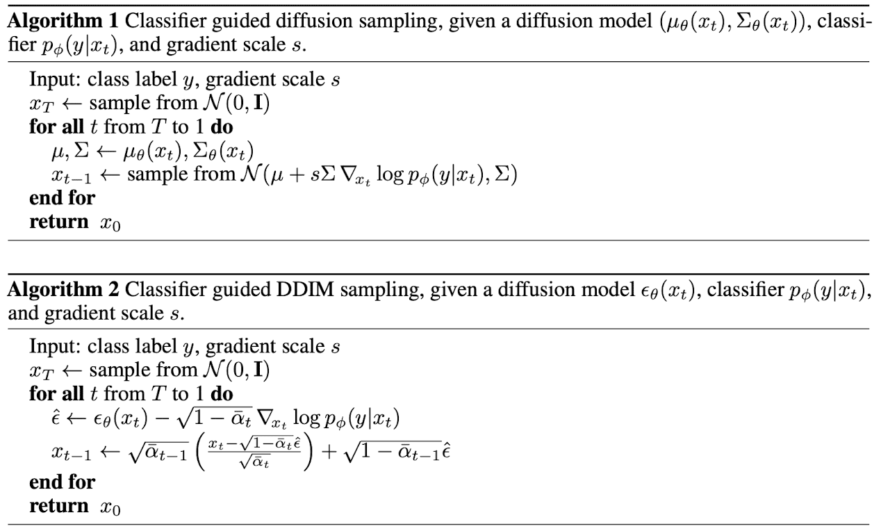
\[\begin{aligned} \hat{\boldsymbol{\epsilon}}_{\theta} (\mathbf{x}_t, t) := \boldsymbol{\epsilon}_\theta(\mathbf{x}_t, t) - \sqrt{1 - \bar{\alpha}_t} \nabla_{\mathbf{x}_t} \log p_{\phi}(y \vert \mathbf{x}_t). \end{aligned}\]The following algorithm shows the class-guided generation of DDPM and DDIM. Practically, it is worthwhile to control the strength of the guidance. To do so, we can add a weight $w$ to the delta parts on both guidances:
\[\begin{aligned} \mathbf{z} \sim \mathcal{N}(\boldsymbol{\mu}_\theta(\mathbf{x}_t, t) + w \cdot \boldsymbol{\Sigma}_\theta(\mathbf{x}_t, t) \mathbf{g}, \boldsymbol{\Sigma}_\theta(\mathbf{x}_t, t)) \end{aligned} \\ \begin{aligned} \hat{\boldsymbol{\epsilon}}_{\theta} (\mathbf{x}_t, t) = \boldsymbol{\epsilon}_\theta(\mathbf{x}_t, t) - w \cdot \sqrt{1 - \bar{\alpha}_t} \nabla_{\mathbf{x}_t} \log p_{\phi}(y \vert \mathbf{x}_t) \end{aligned}\]
In the above derivations, we assumed the unconditional diffusion model \(p_{\theta} (\mathbf{x}_{t-1} \vert \mathbf{x}_t)\), but the authors argue that it can be applied to the coniditional diffusion model \(p_{\theta} (\mathbf{x}_{t-1} \vert \mathbf{x}_t, y)\) in the exact same way. And guiding a conditional model shows better performance than guided unconditional model.
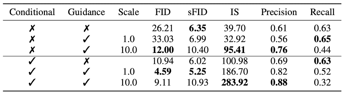
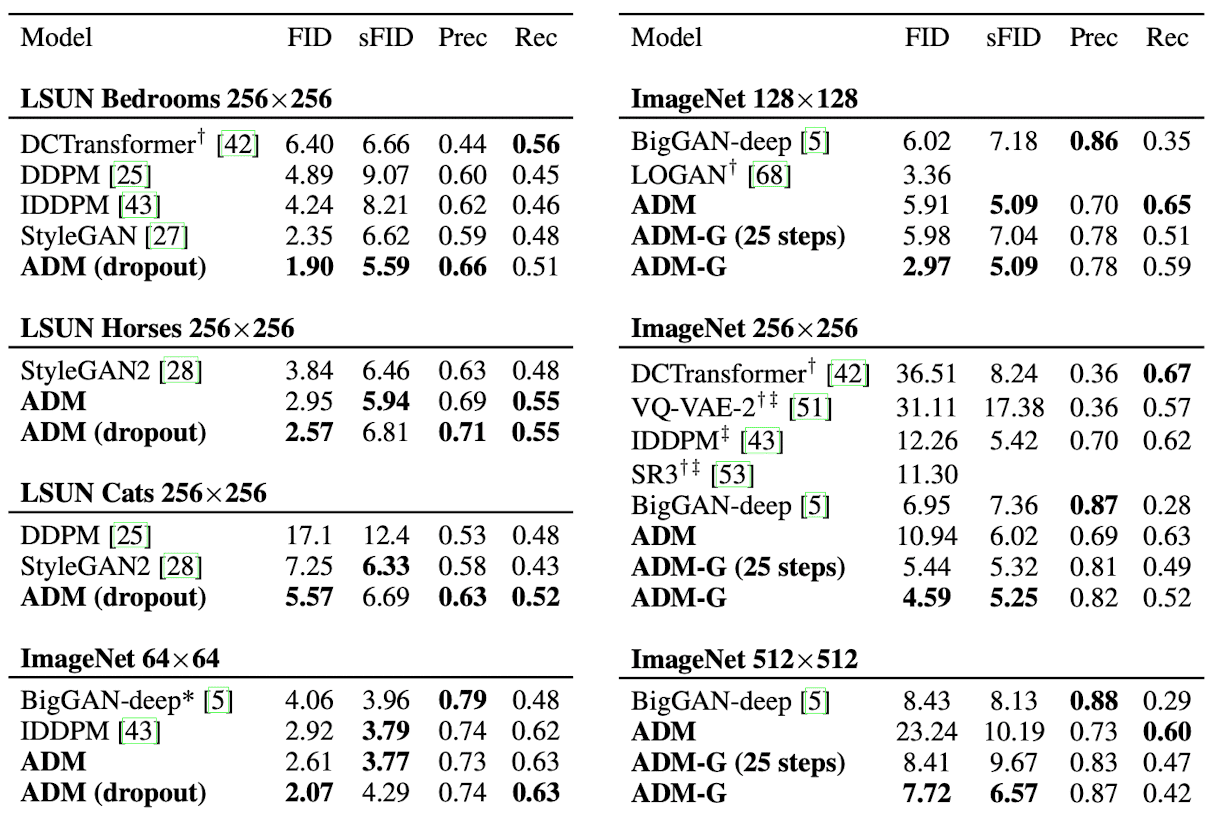
With conditional diffusion model and few modications on the architecture on U-Net, the resulting ablated diffusion model (ADM) and the ADM with classifier guidance (ADM-G) successfully outperform the state-of-the-art GANs in difficult benchamrks (LSUN, ImageNet). The modifications include
- larger depth v.s. width (but holding model size relatively constant)
- increase the number of attention heads
- attention modules with multi-resolution
- using BigGAN residual block for upsampling/downsampling
- Rescaling residual connections with $1 / \sqrt{2}$
- Adaptive Group Normalization (AdaGN)
Classifier-Free Guidance
Algorithm
The main limitation of classfier guidance is that it requires the extra training for the classifier which must be trained on noisy data so it is generally not possible to integrate a pre-trained classifier. Consequently, it adds intricacy to the diffusion model training pipeline.
Ho & Salimans et al. 2021 explored whether classifier guidance can be performed without a classifier. And their classifier-free guidance entirely detached the classifier in the pipeline by jointly training both the conditional and unconditional diffusion models. Recall that the classifier guidance modifies the noise predictor as follows.
\[\begin{aligned} \hat{\boldsymbol{\epsilon}}_{\theta} (\mathbf{x}_t, t) := \boldsymbol{\epsilon}_\theta(\mathbf{x}_t, t) - \sqrt{1 - \bar{\alpha}_t} \nabla_{\mathbf{x}_t} p_{\phi}(y \vert \mathbf{x}_t) \approx - \sqrt{1 - \bar{\alpha}_t} \nabla_{\mathbf{x}_t} [ \log q (\mathbf{x}_t) + w \cdot \log q (y \vert \mathbf{x}_t) ]. \end{aligned}\]Instead of approximating \(\nabla_{\mathbf{x}_t} \log q(y \vert \mathbf{x}_t)\) with the extra classifier ill-sorted with diffusion pipeline, the main idea of classifier-free guidance is eliminating the term with conditional and unconditional diffusion models \(\boldsymbol{\epsilon}_\theta(\mathbf{x}_t, t, y)\) and \(\boldsymbol{\epsilon}_\theta(\mathbf{x}_t, t)\) that approximate \(\nabla_{\mathbf{x}_t} \log q(\mathbf{x}_t \vert y)\) and \(\nabla_{\mathbf{x}_t} \log q(\mathbf{x}_t)\), respectively.
\[\begin{aligned} \nabla_{\mathbf{x}_t} \log q(y \vert \mathbf{x}_t) \propto \nabla_{\mathbf{x}_t} \log q(\mathbf{x}_t \vert y) - \nabla_{\mathbf{x}_t} \log q(\mathbf{x}_t) \end{aligned} \\ \begin{aligned} \therefore \hat{\boldsymbol{\epsilon}}_\theta(\mathbf{x}_t, t, y) &= \boldsymbol{\epsilon}_\theta(\mathbf{x}_t, t, y) + w \big(\boldsymbol{\epsilon}_\theta(\mathbf{x}_t, t, y) - \boldsymbol{\epsilon}_\theta(\mathbf{x}_t, t) \big) \\ &= (w+1) \cdot \boldsymbol{\epsilon}_\theta(\mathbf{x}_t, t, y) - w \cdot \boldsymbol{\epsilon}_\theta(\mathbf{x}_t, t) \end{aligned}\]Note that the guidance can be simply performed with a single neural network for both models by inputting a null token $y = \varnothing$, i.e. \(\boldsymbol{\epsilon}_\theta(\mathbf{x}_t, t) = \boldsymbol{\epsilon}_\theta(\mathbf{x}_t, t, y = \varnothing)\). Consequently, classifier-free guidance can achieve better FID scores than ADM-G and also balance between quality and diversity (i.e., FID and IS).
In summary, the pros and cons of classifier-free guidance against classifier guidance are
(+) The classifier does not need to be trained.
(+) It is more versatile and can be used for any additional information (e.g., text descriptions).
(-) In the generation process, the noise predictor needs to be evaluated twice.
(-) Determining the optimal weight $w$ can be challenging.
Negative Prompting
Tumanyan et al. 2023 show that negative prompting has a more substantial impact than using the empty string $\varnothing$. Max Woolf also finds that negative prompts are crucial for consistently getting good results from the model. Specifically, rather than using the empty string $\varnothing$, negative prompts $p^-$, which indicate elements to be excluded from the generated image, are inserted to the model. This can be formally written as:
\[\hat{\boldsymbol{\epsilon}}_\theta(\mathbf{x}_t, t, y) = (w+1) \cdot \boldsymbol{\epsilon}_\theta(\mathbf{x}_t, t, f_\texttt{txt} (p^+) ) - w \cdot \boldsymbol{\epsilon}_\theta(\mathbf{x}_t, t, f_\texttt{txt} (p^-)) \\\]where $f_\texttt{txt}$ is the text encoder and $p^+$ is the regular user prompt (positive prompt).
GLIDE: Text-Guided Diffusion
Work in progress!
References
[1] Dhariwal & Nichol et al. “Diffusion Models Beat GANs on Image Synthesis.” Advances in neural information processing systems 34 (2021): 8780-8794.
[2] Ho & Salimans et al. “Classifier-free diffusion guidance.” NeurIPS 2021 Workshop
[3] Tumanyan et al. “Plug-and-Play Diffusion Features for Text-Driven Image-to-Image Translation” CVPR 2023
[4] Max Woolf. Stable diffusion 2.0 and the importance of negative prompts for good results. 2023
Leave a comment