
[Generative Model] 2D Prior-based 3D Generation
Initially, most 3D native generative methods were restricted to constrained datasets such as ShapeNet and Objaverse, which contained only fixed object categories with relatively small number of data. Recent advances in text-to-image diffusion models have opened up new possibilities. DreamFusion, Poole et al., 2023, leveraged score distillation sampling (SDS) techniques to transfer prior knowledge from powerful 2D diffusion models into optimizing 3D representations like NeRF, significantly enhancing the quality of text-to-3D synthesis. This paradigm rapidly expanded the scope of diffusion-based approaches from objects to other domains such as scenes and humans.
DreamFusion: Text-to-3D with 2D Diffusion Prior
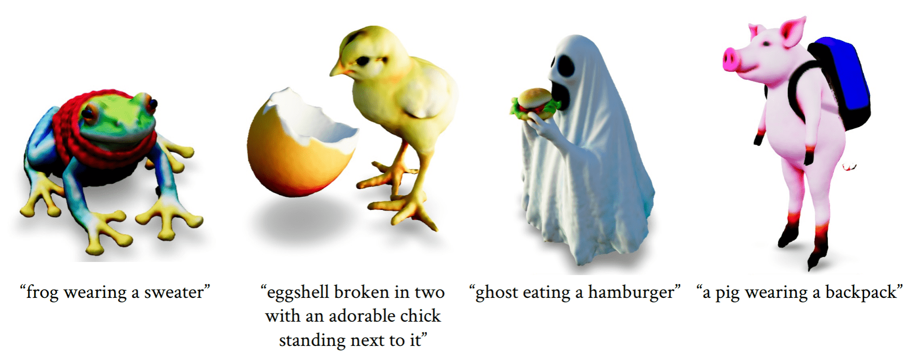
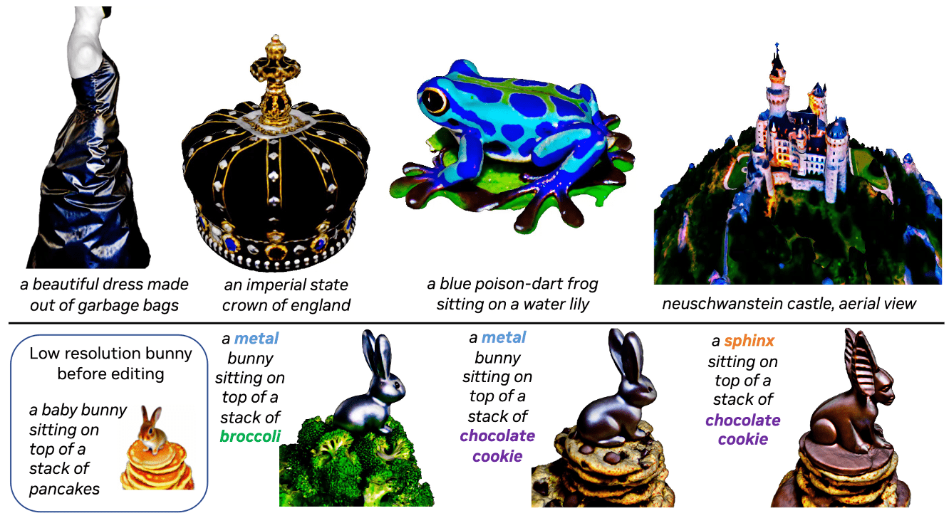
DreamFusion of Poole et al., ICLR 2022 introduced Score Distillation Sampling (SDS), a loss function based on probability density distillation that leverages a pretrained 2D diffusion model to evaluate the plausibility of rendered images. This loss function optimizes a randomly-initialized 3D model (e.g., NeRF) via gradient descent such that its 2D renderings from random angles achieve a low loss. Consequently, the resulting 3D model of the given text can be viewed from any angle, relit by arbitrary illumination, or composited into any 3D environment.
Score Distillation Sampling (SDS)
Let’s revisit the loss function of text-to-image diffusion model conditioned with $y$ using classifier-free guidance \(\boldsymbol{\epsilon_\theta} (\mathbf{x}_t, y, t) \equiv (1 + w) \cdot \boldsymbol{\epsilon_\theta} (\mathbf{x}_t, y, t) - w \cdot \boldsymbol{\epsilon_\theta} (\mathbf{x}_t, \varnothing, t)\):
\[\begin{gathered} \mathcal{L}(\boldsymbol{\theta}) = \mathbb{E}_{t \sim \mathcal{U}[0, 1], \mathbf{x}_0, \boldsymbol{\epsilon}_t \sim \mathcal{N}(\mathbf{0}, \mathbf{I})} [ \Vert \boldsymbol{\epsilon}_t - \boldsymbol{\epsilon_\theta} (\mathbf{x}_t, y, t) \Vert_2^2 ] \\ \begin{aligned} \text{ where } \mathbf{x}_t & = \alpha_t \mathbf{x} + \sigma_t \boldsymbol{\epsilon}_t \\ & := \sqrt{\bar{\alpha}_t} \mathbf{x}_0 + \sqrt{1 - \bar{\alpha}_t} \boldsymbol{\epsilon}_t \quad \text{DDPM} \end{aligned} \end{gathered}\]To create 3D models that look like good images when rendered from random angles $\phi$, we model the image as a differentiable generator $g$ that transforms parameters $\phi$ to create an image $\mathbf{x} = g(\phi)$. In DreamFusion, $g$ is selected to be NeRF, hence $\phi$ is the NeRF parameter. The gradient of $\mathcal{L}$ with respect to $\phi$ in order to train the renderer is given by chain rule:
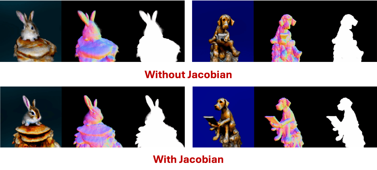
\[\begin{aligned} \nabla_\phi \mathcal{L}(\boldsymbol{\theta}) & = \nabla_{\phi} \mathbb{E}_{t \sim \mathcal{U}[0, 1], \mathbf{x}_0, \boldsymbol{\epsilon}_t \sim \mathcal{N}(\mathbf{0}, \mathbf{I})} [ \Vert \boldsymbol{\epsilon}_t - \boldsymbol{\epsilon_\theta} (\mathbf{x}_t, t) \Vert_2^2 ] \\ & = \mathbb{E}_{t \sim \mathcal{U}[0, 1], \mathbf{x}_0, \boldsymbol{\epsilon}_t \sim \mathcal{N}(\mathbf{0}, \mathbf{I})} \left[ 2 \left( \boldsymbol{\epsilon}_t - \boldsymbol{\epsilon_\theta} (\mathbf{x}_t, y, t) \right) \frac{\partial \boldsymbol{\epsilon_\theta} (\mathbf{x}_t, y, t)}{\partial \mathbf{x}_t} \frac{\partial \mathbf{x}_t}{\partial \mathbf{x}_0} \frac{\partial \mathbf{x}_0}{\partial \phi} \right] \\ & = \mathbb{E}_{t \sim \mathcal{U}[0, 1], \mathbf{x}_0, \boldsymbol{\epsilon}_t \sim \mathcal{N}(\mathbf{0}, \mathbf{I})} \Big[ 2 \alpha_t \underbrace{\left( \boldsymbol{\epsilon}_t - \boldsymbol{\epsilon_\theta} (\mathbf{x}_t, y, t) \right)}_{\textrm{Noise Residual}} \color{red}{\underbrace{\frac{\partial \boldsymbol{\epsilon_\theta} (\mathbf{x}_t, y, t)}{\partial \mathbf{x}_t}}_{\begin{gathered} \textrm{Noise Predictor} \\ \textrm{Jacobian} \end{gathered}}} \color{blue}{\underbrace{\frac{\partial \mathbf{x}_0}{\partial \phi}}_{\begin{gathered} \textrm{Generator} \\ \textrm{Jacobian} \end{gathered}}} \Big] \\ \end{aligned}\]In practice, computing the noise predictor Jacobian term is computationally expensive and is poorly conditioned for small noise levels, given its training to approximate the scaled Hessian of the marginal density. DreamFusion eliminates the noise predictor Jacobian to save on computation time and memory, and therefore the SDS gradient is defined as follows:
\[\begin{aligned} \nabla_\phi \mathcal{L}_{\mathrm{SDS}} & = \mathbb{E}_{t \sim \mathcal{U}[0, 1], \mathbf{x}_0, \boldsymbol{\epsilon}_t \sim \mathcal{N}(\mathbf{0}, \mathbf{I})} \left[ \left( \boldsymbol{\epsilon}_t - \boldsymbol{\epsilon_\theta} (\mathbf{x}_t, y, t) \right) \frac{\partial \mathbf{x}_0}{\partial \phi} \right] \\ & \equiv \nabla_\phi \mathbb{E}_{t, \mathbf{z}_t \vert \mathbf{x}_0} \left[ \frac{\sigma_t}{\alpha_t} \mathrm{KL}(\mathrm{q}_t (\mathbf{z}_t \vert g(\phi); y) \Vert \mathrm{p}_{\boldsymbol{\theta}} (\mathbf{z}_t ; y, t))\right] \end{aligned}\]where \(\mathrm{q}_t (\mathbf{z}_t \vert \mathbf{x}_0; y) = \mathcal{N}(\alpha_t \mathbf{x}_0, \sigma_t^2 \mathbf{I})\) is the forward diffusion and \(\mathrm{p}_{\boldsymbol{\theta}} (\mathbf{z}_t; t)\) denotes the approximate marginal distribution of score function
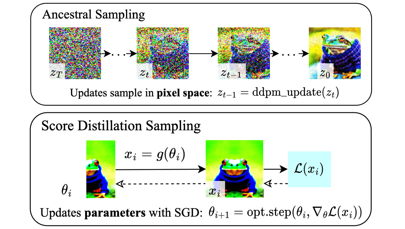
\[\mathbf{s}_\boldsymbol{\theta}(\mathbf{z}_t; t) = −\boldsymbol{\epsilon}_\boldsymbol{\theta} (\mathbf{z}_t; t)/\sigma_t \approx \nabla_{\mathbf{z}_t} \log \mathrm{p}_\boldsymbol{\theta} (\mathbf{z}_t; t).\]Note that the noise in the variational family \(\mathrm{q}_t\) disappears as $t \to 0$ and the mean parameter of the variational distribution $g(\phi)$ becomes the sample of interest. This sampling is named Score Distillation Sampling (SDS) since it predicts the score (noise \(\boldsymbol{\epsilon}_t\)) by the prediction network, using $\nabla \mathcal{L}$, and distills learned knowledge from a pretrained 2D diffusion model, using $\nabla_{\phi} \mathcal{L}_{\textrm{SDS}}$.
Dropping the noise predictor Jacobian is indeed effective. While it takes a similar amount of computation time, it requires twice the VRAM memory.
3D Synthesis
Instead of using the reverse process, DreamFusion samples the outputs by iteratively applying gradient descent from random samples.
- Render the image with NeRF $\mathbf{x}_0 = g(\phi)$
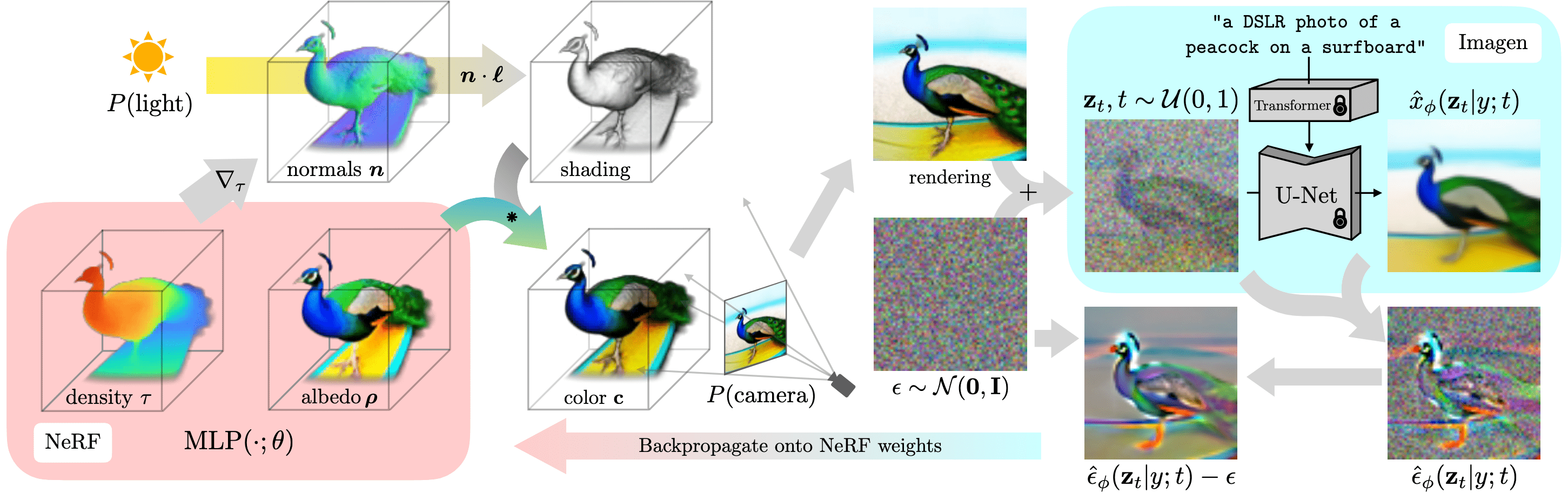
Given NeRF parameter $\phi$ and sampled 3D points $\boldsymbol{\mu}$, compute shading parameters. Specifically, RGB albedo $\boldsymbol{\rho}$ for each point with MLP: $$ (\tau, \boldsymbol{\rho}) = \mathrm{MLP} (\boldsymbol{\mu}; \phi) $$ where $\tau$ is volumetric density. The surface normal vector is computed by $\mathbf{n} = - \nabla_{\boldsymbol{\mu}} \tau / \Vert \nabla_{\boldsymbol{\mu}} \Vert$. With each normal $\mathbf{n}$ and material albedo $\boldsymbol{\rho}$, assuming some point light source with 3D coordinate $\boldsymbol{\ell}$ and color $\boldsymbol{\ell}_\rho$, and an ambient light color $\boldsymbol{\ell}_a$, we render each point along the ray using diffuse reflectance, yielding a color $\mathbf{c}$ for each point: $$ \mathbf{c} = \boldsymbol{\rho} \odot (\boldsymbol{\ell}_p \odot \max (0, \mathbf{n} \cdot (\boldsymbol{\ell} - \boldsymbol{\mu}) / \Vert \boldsymbol{\ell} - \boldsymbol{\mu} \Vert) + \boldsymbol{\ell}_a ) $$ With these values, the volume rendering integral is approximated as in standard NeRF rendering. - Perturb the rendered image $\mathbf{x}_0$
Given the camera pose and light position, render the shaded NeRF model at $64 × 64$ resolution, yielding $\mathbf{x}_0$ and perturb the image with forward diffusion: $$ \mathbf{x}_t = \sqrt{\bar{\alpha}_t} \mathbf{x}_0 + \sqrt{1 - \bar{\alpha}_t} \boldsymbol{\epsilon}_t $$ - Optimization through $\mathcal{L}_{\mathrm{SDS}}$
Perform gradient descent on $\mathcal{L}_{\mathrm{SDS}}$ with respect to the NeRF parameters $\phi$: $$ \nabla_\phi \mathcal{L}_{\mathrm{SDS}} = \mathbb{E}_{t \sim \mathcal{U}[0, 1], \mathbf{x}_0, \boldsymbol{\epsilon}_t \sim \mathcal{N}(\mathbf{0}, \mathbf{I})} \left[ \left( \boldsymbol{\epsilon}_t - \boldsymbol{\epsilon_\theta} (\mathbf{x}_t, y, t) \right) \frac{\partial \mathbf{x}_0}{\partial \phi} \right] $$
Magic3D: High-Resolution for Text-to-3D
DreamFusion has two inherent limitations, leading to low-quality 3D models with a long processing time:
- extremely slow optimization of NeRF
- low-resolution image space supervision on NeRF,
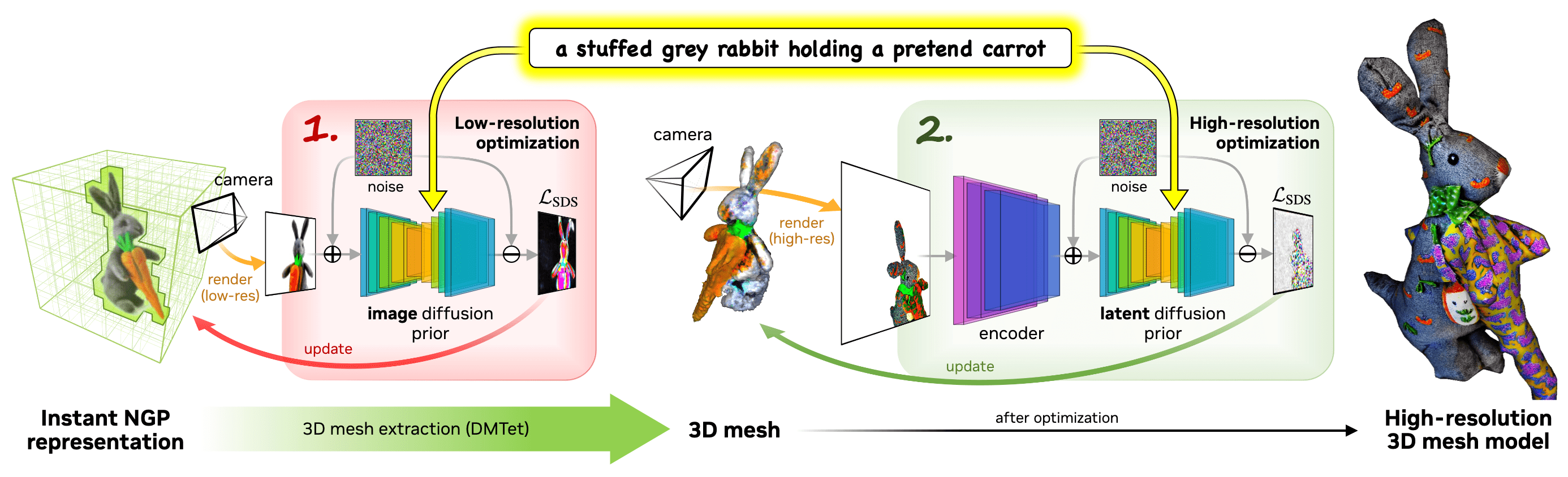
To mitigate these issues, Lin et al. CVPR 2023 introduced Magic3D that utilizes two-stage optimization framework that extracts a coarse mesh in the first stage, and then texture the mesh in the second stage.
Specifically, Magic3D adopts end-to-end, coarse-to-fine optimization approach that uses multiple diffusion priors at different resolutions to optimize the 3D representation, enabling the generation of both view-consistent geometry as well as high-resolution details.
- Optimization of coarse neural field representation
In the initial stage, Magic3D finds the geometry and textures through the optimization of coarse NeRF representation by SDS with diffusion prior defined on low resolution $64 \times 64$: $$ \nabla_\phi \mathcal{L}_{\mathrm{SDS}} = \mathbb{E}_{t \sim \mathcal{U}[0, 1], \mathbf{x}_0, \boldsymbol{\epsilon}_t \sim \mathcal{N}(\mathbf{0}, \mathbf{I})} \left[ \left( \boldsymbol{\epsilon}_t - \boldsymbol{\epsilon_\theta} (\mathbf{x}_t, y, t) \right) \frac{\partial \mathbf{x}_0}{\partial \phi} \right] $$ For memory- and compute-efficient scene representation, Magic3D utilizes the hash grid representation of Instant-NGP, which can drastically accelerate the optimization of coarse scene models while maintaining quality. - Optimization of fine textured meshes representation
To fine-tune the coarse scene model with high-resolution diffusion priors at high resolution $512 \times 512$, Magic3D adopts 3D mesh representation that enables render high-resolution images in real-time with differentiable rasterization. Formally, we represent the 3D shape using deformable tetrahedral grid $(V_T, T)$, where $V_T$ is the vertices in the grid $T$. Each vertex $\mathbf{v}_i \in V_T \subset \mathbb{R}^3$ contains SDF value $s_i \in \mathbb{R}$ and deformation $\Delta \mathbf{v}_i \in \mathbb{R}^3$ of the vertex from its initial canonical coordinate. (Note that if all $\Delta \mathbf{v}_i$ are fixed, the representation is equivalent to voxel-grid.)
Then, surface meshes are extracted from the SDF using a differentiable marching tetrahedra algorithm, and Magic3D utilizes the neural color field as a volumetric texture representation for textures. During optimization, Magic3D renders the extracted surface mesh into high-resolution images using a differentiable rasterizer, increasing the focal length to zoom in on object details. Then both $s_i$ and $\Delta \mathbf{v}_i$ for each vertex $\mathbf{v}_i$ are optimized via backpropagation of the high-resolution SDS gradient.
ProlificDreamer
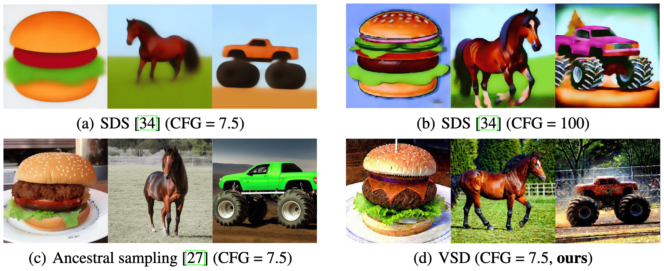
Score Distillation Sampling (SDS) algorithm optimizes a single 3D representation such that the image rendered from any view maintains a high likelihood as evaluated by the diffusion model, and has shown great promise in text-to-3D generation. However, it is known that SDS often suffers from over-saturation, over-smoothing, and low-diversity problems. Moreover, SDS does not converge well without a high CFG weight (e.g., $w = 400$) and thus suffers from model collapse. To address these issues, Wang et al. 2023 proposed variational score distillation (VSD) with key insight that multiple 3D scenes can potentially align with one prompt. To capture such phenomenon, VSD minimizes the SDS loss for the multiple samples of the NeRF parameters $\phi$, and also finetunes the diffusion model with the LoRA technique.
Variational Score Distillation (VSD)
Specifically, Variational Score Distillation (VSD) treats the corresponding the rendered scene $\mathbf{x}_0 = g(\phi, c)$ given the camera $c$ with the rendering function (e.g., NeRF) $g(\cdot, c)$ parameterized by parameter $\phi \sim \mu(\phi \vert y)$, given textual prompt $y$, as a random variable with distribution $\mathrm{q}_0^\mu (\mathbf{x}_0 \vert c, y)$ instead of a single point as in SDS. VSD optimizes a distribution of 3D representations such that the distribution induced on images rendered from all views aligns as closely as possible, in terms of KL divergence, with $\mathrm{p}_0 (\mathbf{x}_0 \vert y^c)$ defined by the pretrained text-to-image diffusion model with the view-dependent prompt $y^c$:
\[\underset{\mu}{\min} \; \mathrm{KL}(\mathrm{q}_0^\mu (\mathbf{x}_0 \vert c, y) \Vert \mathrm{p}_0 (\mathbf{x}_0 \vert y^c))\]To circumvent the intractability of $\mathrm{p}_0$, ProlificDreamer rather solves the following equivalent problem:
\[\begin{gathered} \mu^* := \underset{\mu}{\arg \min} \; \mathbb{E}_{t, c} \left[ \frac{\sigma_t}{\alpha_t} \mathrm{KL} (\mathrm{q}_t^\mu (\mathbf{x}_0 \vert c, y) \Vert \mathrm{p}_t (\mathbf{x}_t \vert y^c)) \right] \\ \begin{aligned} \text{where } \mathrm{q}_t^\mu (\mathbf{x}_t \vert c, y) & := \int \mathrm{q}_0^\mu (\mathbf{x}_0 \vert c, y) \mathrm{p}_{t0} (\mathbf{x}_t \vert \mathbf{x}_0) \mathrm{d}\mathbf{x}_0 \\ \mathrm{p}_t (\mathbf{x}_t \vert c, y) & := \int \mathrm{p}_0 (\mathbf{x}_0 \vert c, y) \mathrm{p}_{t0} (\mathbf{x}_t \vert \mathbf{x}_0) \mathrm{d}\mathbf{x}_0 \end{aligned} \end{gathered}\]with forward diffusion $\mathrm{p}_{t0} (\mathbf{x}_t \vert \mathbf{x}_0) = \mathcal{N}(\mathbf{x}_t \vert \alpha_t \mathbf{x}_0, \sigma_t^2 \mathbf{I})$. Compared with SDS that optimizes for the single point $\phi$, VSD optimizes for the whole distribution $\phi \sim \mu$.
\[\begin{aligned} & \text{SDS}: \phi^* := \underset{\color{red}{\phi}}{\arg \min} \; \mathbb{E}_{t, c} \left[ \frac{\sigma_t}{\alpha_t} \mathrm{KL} (\mathrm{q}_t^\phi (\mathbf{x}_0 \vert c, y) \Vert \mathrm{p}_t (\mathbf{x}_t \vert y^c)) \right] \\ & \text{VSD}: \mu^* := \underset{\color{blue}{\mu}}{\arg \min} \; \mathbb{E}_{t, c} \left[ \frac{\sigma_t}{\alpha_t} \mathrm{KL} (\mathrm{q}_t^\mu (\mathbf{x}_0 \vert c, y) \Vert \mathrm{p}_t (\mathbf{x}_t \vert y^c)) \right] \end{aligned}\]Update Rule for VSD
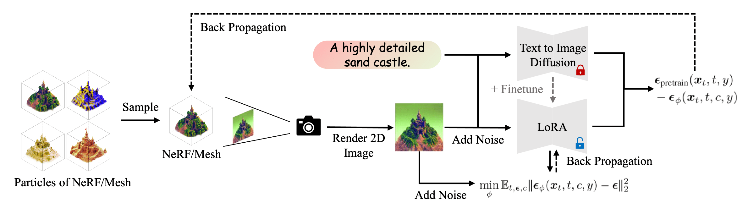
To solve the optimization problem efficiently, VSD maintains a set of 3D parameters \(\{ \phi_i \}_{i=1}^n\) to represent the 3D distribution. We derive a novel gradient-based update rule for the particles via the Wasserstein gradient flow and guarantee that the particles will be samples from the desired distribution when the optimization converges.
Starting from an initial distribution $\mu_0$, denote the Wasserstein gradient flow of the optimization problem in the distribution space at each time $\tau \geq 0$ as $\{ \mu_\tau \}_{\tau \geq 0}$ with $\mu_{\infty} = \mu^*$. Then, $\phi_\tau \sim \mu_\tau$ can be sampled by firstly sampling $\phi_0 \sim \mu_0 (\cdot \vert y)$ and then simulating the following ODE: $$ \frac{\mathrm{d} \phi_\tau}{\mathrm{d} \tau} = - \mathbb{E}_{t, \boldsymbol{\epsilon}, c} \left[ w(t) \left( \underbrace{- \sigma_t \nabla_{\mathbf{x}_t} \log \mathrm{p}_t (\mathbf{x}_t \vert y^c)}_{\textrm{score of noisy real images}} - (\underbrace{- \sigma_t \nabla_{\mathbf{x}_t} \log \mathrm{q}_t^{\mu_\tau} (\mathbf{x}_t \vert c, y)}_{\textrm{score of noisy rendered images}}) \right) \frac{\partial g (\phi_\tau, c)}{\partial \phi_\tau} \right] $$ where $\mathrm{q}_t^{\mu_\tau}$ is the corresponding noisy distribution at diffusion time $t$ w.r.t. $\mu_\tau$ at ODE time $\tau$.
Therefore, VSD requires estimating the score function of the distribution on diffused real and rendered images, which can be approximated by the pre-trained diffusion model \(\boldsymbol{\epsilon}_{\mathrm{pretrain}} (\mathbf{x}_t, t, y^c)\) and noise prediction network \(\boldsymbol{\epsilon}_{\boldsymbol{\theta}} (\mathbf{x}_t, t, c, y)\), respectively:
\[\min_{\boldsymbol{\theta}} \sum_{i=1}^n \mathbb{E}_{t\sim\mathcal{U}(0,1),\boldsymbol{\epsilon}\sim\mathcal{N}(\mathbf{0},\mathbf{I}),c \sim p(c)}\left[ \Vert \boldsymbol{\epsilon}_{\boldsymbol{\theta}}(\mathbf{x}_t,t,c,y) - \boldsymbol{\epsilon} \Vert_2^2 \right] \text{ where } \mathbf{x}_t = \alpha_t g(\phi^{(i)},c) + \sigma_t \boldsymbol{\epsilon}\]where \(\boldsymbol{\epsilon}_{\boldsymbol{\theta}}\) can be efficiently and effectively implemented by LoRA of the pretrained diffusion model. The final algorithm alternatively updates the particles $\phi_i$ and score function \(\boldsymbol{\epsilon}_{\boldsymbol{\theta}}\):
\[\begin{gathered} \phi^{(i)} \leftarrow \phi^{(i)} - \eta \nabla_\phi \mathcal{L}_{\textrm{VSD}} (\phi^{(i)}) \\ \text{ where } \nabla_\phi \mathcal{L}_{\textrm{VSD}} (\phi^{(i)}) = \mathbb{E}_{t, \boldsymbol{\epsilon}, c} \left[ w(t) \left(\boldsymbol{\epsilon}_{\mathrm{pretrain}}(\mathbf{x}_t,t,y^c) - \boldsymbol{\epsilon}_{\boldsymbol{\theta}}(\mathbf{x}_t,t,c,y) \right) \frac{\partial g(\phi, c)}{\partial \phi} \right] \end{gathered}\]
Theoretically, SDS is a special case of VSD with single-point Dirac distribution $\mu(\phi \vert y) = \delta(\phi - \phi^{(1)})$ as the variational distribution. Since VSD employs multiple points and also learns a parametric score function \(\boldsymbol{\epsilon}_{\boldsymbol{\theta}}\) for each points, VSD may potentially offer superior generalization ability and provide more accurate updating directions in low-density regions.
Moreover, since VSD aims to sample $\phi$ from the optimal $\mu^*$ defined by the pretrained model \(\boldsymbol{\epsilon}_{\mathrm{pretrain}}\), the results of tuning the CFG in \(\boldsymbol{\epsilon}_{\mathrm{pretrain}}\) for 3D sampling by VSD closely resemble those of 2D sampling via conventional ancestral sampling techniques. Consequently, VSD can modulate CFG with the same flexibility as traditional text-to-image methodologies.
References
[1] Poole et al. “DreamFusion: Text-to-3D using 2D Diffusion”, ICLR 2023
[2] Lin et al. “Magic3D: High-Resolution Text-to-3D Content Creation”, CVPR 2023 Highlight
[3] Wang et al. “ProlificDreamer: High-Fidelity and Diverse Text-to-3D Generation with Variational Score Distillation”, NeurIPS 2023 (Spotlight)
[4] Liu et al. “A Comprehensive Survey on 3D Content Generation”, arXiv:2402.01166
Leave a comment