[Generative Model] Wasserstein GAN

Wasserstein Distance

Let $M$ be a set and a mapping $\delta: M \times M \to [0, \infty)$ be a metric. With these, define a metric space $(M, \delta)$. Denote the set of all joint distributions $\gamma$ whose marginals are $\mu$ and $\nu$ by $\Pi(\mu, \nu)$. Note that this collection is not an empty set since it contains a product measure $\mu \times \nu$. (in terms of probability theory, a joint distribution that two marginal distributions are independent.) Hence, for all events $E \subset M \times M$ and $F \subset M$,

\[\begin{aligned} \gamma (E) & \in [0, 1] \\ \gamma(F \times M) & = \mu (F) = \int_F \; d\mu \\ \gamma(M \times F) & = \nu (F) = \int_F \; d\nu \end{aligned}\]

We are now interested in measuring “distance” between two distributions $\mu$ and $\nu$. Wasserstein distance, or Kantorovich–Rubinstein metric measures the distance by the expectation of random distance $\delta (X, Y)$ where $X \sim \mu$ and $Y \sim \nu$.

$\color{blue}{\mathbf{Definition.}}$ Wasserstein distance
We define the Wasserstein distance between two distributions $\mu$ and $\nu$ as $$ \begin{aligned} W (\mu, \nu)= \inf _{\gamma \in \Pi (\mu, \nu)} \mathbb{E}_{(X, Y) \sim \gamma} [\delta( X, Y )] \end{aligned} $$ For $p \in [1, +\infty]$, it can be generalized into Wasserstein $p$-distance as $$ \begin{aligned} W_p (\mu, \nu)= \left( \inf _{\gamma \in \Pi (\mu, \nu)} \mathbb{E}_{(X, Y) \sim \gamma} [\delta( X, Y )^p] \right)^{1/p} \end{aligned} $$ where ${\displaystyle W_{\infty }(\mu, \nu)}$ is defined to be a supremum norm.

Intuitively, if each distribution is envisioned as a unit amount of earth (soil) stacked on $M$, the metric represents the minimum “cost” of transforming one pile into the other. This cost is assumed to be the quantity of earth that needs to be moved, multiplied by the mean distance it has to be moved. Thus Wasserstein distance is usually referred to as Earth Mover’s (EM) distance.

Kantorovich-Rubinstein Theorem

In general, the infimum in the distance is highly intractable; it is impossible to compute $W (\mu, \nu)$ by the collection $\Pi (\mu, \nu)$, but Kantorovich-Rubinstein theorem gives us circumvention for computation that $W (\mu, \nu)$ equals to the dual norm of Lipschitz norm between $\mu$ and $\nu$.

Recall that Lipschitz norm of function $f: M \to \mathbb{R}$ defined on metric space $(M, \delta)$ is defined by

\[\begin{aligned} \lVert f \rVert_L:=\sup \{|f(x)-f(y)| / \delta(x, y): x \neq y \text { in } M\} \end{aligned}\]

Then the dual norm of Lipschitz norm is defined by

\[\begin{aligned} \rho(\mu, \nu):=\lVert \mu-\nu \rVert_L^* & :=\sup \left\{\int_S f(x) \; d(\mu-\nu)(x):\lVert f \rVert_L \leq 1\right\} \\ & =\frac{1}{K} \sup \left\{\int_S f(x) \; d(\mu-\nu)(x):\lVert f \rVert_L \leq K\right\} \end{aligned}\]

$\color{red}{\mathbf{Theorem.}}$ Kantorovich-Rubinstein Theorem
For any separable metric space $(M, \delta)$ and any two distributions $\mu$ and $\nu$ in $\mathcal{P}_1 (M)$, $$ \begin{aligned} W (\mu, \nu) = \rho(\mu, \nu). \end{aligned} $$ If $M$ is complete, then there exists a distribution $\gamma$ in $\Pi (\mu, \nu)$ such that $\int_{M \times M} \delta (x, y) \; d\gamma(x, y) = W (\mu, \nu)$, so that the infimum in the definition of $W (\mu, \nu)$ is attained.

Those who are interested in the proof of theorem, please see §11.8 of [1]. It requires the understanding of advanced measure theory. Also, this blog post provides neat introduction to the proof of theorem.

Wasserstein-GAN (WGAN)

Algorithm

Wasserstein GAN formulates its loss function by

\[\begin{aligned} W\left(\mathbb{P}_r, \mathbb{P}_g\right) & =\inf _{\gamma \sim \mathcal{J}\left(\mathbb{P}_r, \mathbb{P}_g\right)} \mathbb{E}_{(X, Y) \sim \gamma}[\lVert X-Y \rVert] \\ & =\frac{1}{K} \sup _{\lVert f \rVert_L \leq K} \mathbb{E}_{X \sim \mathbb{P}_r}[f(X)]-\mathbb{E}_{Y \sim \mathbb{P}_g}[f(Y)] \end{aligned}\]

for two distributions \(\mathbb{P}_r\) and \(\mathbb{P}_g\). To approximate the function $f$ that solves the optimization problem, it trains a critic (discriminator) neural network $f_w$ parameterized with weights $w$ lying in a compact space $\mathcal{W}$. Therefore, the critic no longer serves as a direct critic for discriminate fake samples from real ones. Instead, it is trained to learn a Lipschitz continuous function that estimates the Wasserstein distance. During training, critic $f_w$ is optimized to maximize the loss function to estimate the Wasserstein distance, and the generator $G_\theta$ is optimized to minimize the loss function (i.e. approximation of Wasserstein distance) to approach the distribution of real data.

The big issue is to sustain the Lipschitz continuity of $f_w$ during the training. Although compact space $\mathcal{W}$ does not always ensure the Lipschitz continuity of neural network, for instance,

\[\begin{aligned} f_w(x) = \begin{cases} \sigma\left(\frac{x}{w}\right) = 1/(1+\exp(-x/w)) & w \ne 0 \\ \mathrm{sgn}(x) & w = 0 \end{cases} \end{aligned}\]

but it holds for a typical network $f_w^H$ that is recursively defined by

\[\begin{aligned} f_w^{(0)}(x) = x \qquad f_w^{(\ell)}(x) = \sigma_\ell(W_\ell f_w^{(\ell-1)}(x) + b_\ell) \end{aligned}\]

where $w$ contains all of the parameters $W_\ell$, $b_\ell$ for each layer $\ell$ and each $\sigma_\ell$ is some fixed Lipschitz activation function. It is well-known fact that most activation functions such as ReLU, leaky ReLU, softplus, tanh, sigmoid, arctan or softsign, as well as max-pooling, have a Lipschitz constant equal to 1. Also, other common neural network layers such as dropout, batch normalization and other pooling methods all have simple and explicit Lipschitz constants. [5] Then we can easily show that

\[\begin{aligned} \lVert f_w^{(H)} \rVert_L \le \lVert \sigma_{H} \rVert_L \; \lVert W_H \rVert_\mathrm{op} \lVert f_w^{(H-1)} \rVert_L \le \cdots \le \prod_{\ell=1}^H \lVert \sigma_{\ell} \rVert_L \; \lVert W_\ell \rVert_\mathrm{op}. \end{aligned}\]

Since $\mathcal{W}$ is compact, then weight is bounded, i.e. there exists a constant $M > 0$ such that $\lVert W_\ell \rVert_{\mathrm{op}} \leq M$ for every $w \in \mathcal{W}$. Thus, for any $w \in \mathcal{W}$, we have

\[\begin{aligned} \lVert f_w^{(H)} \rVert_L \le \prod_{\ell=1}^H \lVert \sigma_{\ell} \rVert_L \; \lVert W_\ell \rVert_\mathrm{op} \le M^H \prod_{\ell=1}^H \lVert \sigma_{\ell} \rVert_L \end{aligned}\]

In order to have parameters $w$ lie in a compact space $\mathcal{W}$, WGAN simply clamps the weights to a fixed box (say $\mathcal{W} = [0.01, 0.01]^H$) after each gradient update. The following pseudocode shows the WGAN procedure:

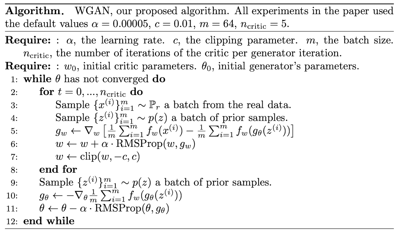
$\mathbf{Fig\ 1.}$ Algorithm of Wasserstein generative adversarial network. (source: [2])

Background

The most fundamental and important criterions of distances that we should consider for objectives are

• continuity of $\theta \to P_{\theta}$
  • if the parameter $\theta_t$ converges to the optimal $\theta$, the parametric distribution $P_{\theta_t}$ induced by $\theta_t$ must converge to the optimal distribution $P_\theta$.
• impact on the convergence
  • In general, there is a tendency that a distance $\rho$ induces a weaker topology when it makes it easier for a sequence of distribution to converge.
  • We say the topology induced by $\rho$ is weaker than that induced by $\rho^\prime$ when the set of convergent sequences under $\rho$ contains that under $\rho^\prime$.
• well-definedness (e.g. on low-dimensional manifolds)
  • There must exist a solution to the optimization problem for minimizing distance and must be tractable.
  • The dimension of space of data in real-world is usually lower than the dimension of the ambient space (manifold hypotheses), thus the distances and divergences must be viable on that.
  • In general, for example, KL divergence is not defined or simply infinite on low-dimensional manifolds.

On top of these, the authors of [2] demonstrate the advantages of Wasserstein distance between other distances for two probability measure $\mu$ and $\nu$:

• Total Variation (TV) distance $$ \begin{aligned} \text{TV} (\mu, \nu) = \sup _{A \in \mathcal{B}} | \mu (A) - \nu (A) | \end{aligned} $$ where $\mathcal{B}$ stands for the collection of all the Borel subsets of $\chi$.
• Kullback-Leibler (KL) divergence $$ \begin{aligned} \text{KL} (\mu \Vert \nu) = \int_\chi \log \left( \frac{\mu}{\nu} \right) \; d\mu \end{aligned} $$ Note that it is assymetric and possibly infinite when there are points such that $\mu(A) = 0$ and $\nu (A) > 0$.
• Jensen-Shannon (JS) divergence $$ \begin{aligned} \text{JS} (\mu, \nu) = \frac{1}{2} \text{KL} \left( \mu \lVert \frac{\mu + \nu}{2} \right) + \frac{1}{2} \text{KL} \left(\nu \rVert \frac{\mu + \nu}{2}\right) \end{aligned} $$ Note that it is symmetrical and always defined.

and proposed Wasserstein GAN.

Continuity and A.E. differentiability

First of all, the Wasserstein distance is a continuous loss function on $\theta$ (and even differentiable almost everywhere for some case) under mild assumptions. Here is our regularity assumption for the next theorem:

$\color{black}{\mathbf{Assumption.}}$ Let $g: \mathbb{R}^d \times \mathcal{Z} \to \chi$ be locally Lipschitz between finite dimensional vector spaces. We say that $g$ satisfies regularity condition for a certain distribution $p$ over $\mathcal{Z}$ if there are local Lipschitz constants $L(\theta, z)$ such that $$ \begin{aligned} \mathbb{E}_{z \sim p} [L(\theta, z)] < +\infty. \end{aligned} $$

Before we start, recall that every (locally) Lipschitz continuous function is differentiable almost everywhere. This is ensured by Radamacher’s theorem, and we will use that result for our proof of theorem.

$\color{red}{\mathbf{Theorem.}}$ Continuity and a.e. differentiability of Wasserstein distance
Let $\chi = (M, \delta)$ be a compact metric space. Let $\mu$ be a fixed distribution over $\chi$. Let $Z$ be a random variable over another space $\mathcal{Z}$. Let $G: \mathbb{R}^d \times \mathcal{Z} \to \chi$ be a function, and denote $G_\theta (z) = G(\theta, z)$. Then, let $\mu_\theta$ be the distribution of $G_\theta(Z)$.

1. If $G$ is continuous in $\theta$, so is $W(\mu, \mu_\theta)$.
2. If $G$ is locally Lipschitz and satisfies regularity condition, then $W (\mu, \mu_\theta)$ is continuous everywhere, and differentiable almost everywhere.

However, these are all false for the Jensen-Shannon divergence and KL divergences.

$\mathbf{Proof.}$

(1) Let $\theta \in \mathbb{R}^d$ and $\theta^\prime \in \mathbb{R}^d$ be 2 parameters. Let $\gamma \in \Pi(\mu_\theta, \mu_{\theta^\prime})$ be the distribution of joint $(G_\theta(Z), G_{\theta^\prime} (Z))$.

By the definition of the Wasserstein distance, as $(X, Y) \sim \gamma = (G_\theta(Z), G_{\theta^\prime} (Z))$, we have

\[\begin{aligned} W(\mu_{\theta}, \mu_{\theta^\prime}) & \leq \mathbb{E}_{(X, Y) \sim \gamma} [\delta (X, Y)] \\ & = \mathbb{E}_{Z \sim \mathcal{Z}} [\delta (G_{\theta} (Z), G_{\theta^\prime} (Z))]. \end{aligned}\]

If $G$ is continuous in $\theta$, then \(\lim _{\theta \to \theta^\prime} G_{\theta} (z) = G_{\theta^\prime} (z)\) pointwisely. In other words, \(\lim _{\theta \to \theta^\prime} \delta (G_{\theta} (z), G_{\theta^\prime} (z)) = 0\) pointwisely.

Note that $\chi$ is compact. Since metric $\delta$ is continuous function, it is uniformly bounded by $M \geq 0$ on $\chi$. Therefore $\delta (G_{\theta} (z), G_{\theta^\prime} (z)) \leq M$ for all $\theta$ and $z$ uniformly. By bounded convergence theorem (or dominated convergence theorem),

\[\begin{aligned} W(\mu_\theta, \mu_{\theta^\prime}) & \leq \lim _{\theta \to \theta^{\prime}} \mathbb{E}_{Z \sim \mathcal{Z}} [\delta (G_{\theta} (Z), G_{\theta^\prime} (Z))] \\ & = \mathbb{E}_{Z \sim \mathcal{Z}} [\lim _{\theta \to \theta^{\prime}} \delta (G_{\theta} (Z), G_{\theta^\prime} (Z))] \\ & = 0. \end{aligned}\]

Hence, we now prove the continuity of $W(\mu, \mu_{\theta})$:

\[\begin{aligned} \lim _{\theta \to \theta^\prime} | W(\mu, \mu_{\theta}) - W(\mu, \mu_{\theta^\prime}) | \leq \lim _{\theta \to \theta^\prime} | W(\mu_{\theta}, \mu_{\theta^\prime}) | = 0. \end{aligned}\]

(2) Let $G$ be locally Lipschitz. In other words, for any point $(\theta, z)$, there exists a constant $L(\theta, z)$ and an open set $U$ that contains $(\theta, z)$ where for every $(\theta^\prime, z^\prime) \in U$,

\[\begin{aligned} \delta(G_{\theta} (z) - G_{\theta^\prime} (z)) \leq L(\theta, z) \times (\delta(\theta, \theta^\prime) + \delta(z, z^\prime)). \end{aligned}\]

By taking expectations on both sides and setting $z^\prime = z$,

\[\begin{aligned} \mathbb{E}_{Z \sim \mathcal{Z}} [\delta (G_\theta (Z) - G_{\theta^\prime} (Z))] \leq \mathbb{E}_{Z \sim \mathcal{Z}} [L(\theta, Z)] \times \delta(\theta, \theta^\prime) \end{aligned}\]

whenever $(\theta^\prime, z) \in U$. Define

\[\begin{aligned} U_{\theta} = \{ \theta^\prime : (\theta^\prime, z) \in U \} \end{aligned}\]

Note that it is open as the section of open set is also open. Furthermore, by regularity assumption, we can define \(L(\theta) = \mathbb{E}_{Z \sim \mathcal{Z}} [L(\theta, Z)]\) and thus show that $W(\mu, \mu_\theta)$ is locally Lipschitz:

\[\begin{aligned} | W(\mu, \mu_\theta) - W(\mu, \mu_{\theta^\prime}) | \leq W(\mu_{\theta}, \mu_{\theta^\prime}) \leq L(\theta) \times \delta(\theta, \theta^\prime) \end{aligned}\]

for all $\theta^\prime \in U_\theta$. Hence, it is continuous everywhere and by Radamacher’s theorem it is differentiable almost everywhere.

\[\tag*{$\blacksquare$}\]

$\color{blue}{\mathbf{Corollary.}}$ Let $G_\theta$ be any feedforward neural network parameterized by $\theta$ and $p(z)$ be the prior distribution over $z$ such that $\mathbb{E}_{z \sim p(z)} [\lVert z \rVert] < \infty$ (e.g. Gaussian, uniform, etc.). Then the regularity assumption is satisfied and therefore $W(\mu, \mu_{\theta})$ is continuous everywhere and differentiable almost everywhere.
Here, a feedforward neural network is a function composed by affine transformations and pointwise nonlinearities which are smooth ($C^{\infty}$) Lipschitz functions such as the sigmoid, tanh, etc. The statement is also true for ReLU.

$\mathbf{Proof.}$

Here, we use the fact that continuously differentiable implies locally Lipschitz, which implies functions in $C^\infty$, i.e. smooth functions are all locally Lipschitz. Given $x_0$ and $\varepsilon > 0$, by the continuity of $f^\prime$, there exists an open ball $U$ of $x_0$ such that $\lVert f^\prime (x) − f^\prime (x_0) \rVert \leq \varepsilon$ for all $x \in U$. It follows that $\lVert f^\prime(x) \rVert \leq \lVert f^\prime (x_0) \rVert + \varepsilon$ in $U$. Now the Mean Value Theorem implies that $f$ is Lipschitz on $U$.

Note that it does not have to be globally Lipschitz in general, as the one-dimensional example $f(x) = x^2$ shows.

Now, we begin with the case of smooth nonlinearities. Since $G$ is $C^1$ as a function of $(\theta, z)$, for any fixed $(\theta, z)$ we have $L(\theta, z) \leq \lVert \nabla_{\theta, z} G_\theta (z) \rVert + \varepsilon$. Therefore, it suffices to show that

\[\begin{aligned} \mathbb{E}_{z \sim p} [\lVert \nabla_{\theta, z} G_\theta (z) \rVert] < \infty. \end{aligned}\]

Let $H$ be the number of layers. We know that $\nabla_z G_\theta (z) = \prod_{k=1}^H W_k D_k$ where $W_k$ are the weight matrices and $D_k$ are the diagonal Jacobians of the diagoanl Jacobians of the nonlinearities.

Let $f_{i:j}$ be the application of layers $i$ to $j$ inclusively (e.g. $G_\theta = f_{1: H}$). Then,

\[\begin{aligned} \nabla_{W_k} G_\theta (z) = ((\prod_{i=k+1}^H W_i D_i) D_k) f_{1:k-1} (z). \end{aligned}\]

Note that if $L$ is the Lipschitz constant of the nonlinearity, its derivative is also bounded by $L$, i.e. $\lVert D_i \rVert \leq L$. Also, $\lVert f_{1: k - 1} (z) \rVert \leq \lVert z \rVert L^{k-1} \prod_{i=1}^{k-1} W_i$. Finally, then we have

\[\begin{aligned} \left\|\nabla_{z, \theta} g_\theta(z)\right\| & \leq\left\|\prod_{i=1}^H W_i D_i\right\|+\sum_{k=1}^H\left\|\left(\left(\prod_{i=k+1}^H W_i D_i\right) D_k\right) f_{1: k-1}(z)\right\| \\ & \leq L^H \prod_{i=H}^K\left\|W_i\right\|+\sum_{k=1}^H\|z\| L^H\left(\prod_{i=1}^{k-1}\left\|W_i\right\|\right)\left(\prod_{i=k+1}^H\left\|W_i\right\|\right) \end{aligned}\]

Therefore

\[\begin{aligned} \mathbb{E}_{z \sim p} [\left\|\nabla_{z, \theta} g_\theta(z)\right\|] \leq L^H (\prod_{i=1}^H \| W_i \|) + \sum_{k=1}^H \mathbb{E}_{z \sim p} [\|z\|] L^H\left(\prod_{i=1}^{k-1}\left\|W_i\right\|\right)\left(\prod_{i=k+1}^H\left\|W_i\right\|\right) < \infty \end{aligned}\]

The statement is also true for ReLU, but the proof is more technical (even though very similar) so it is omitted.

\[\tag*{$\blacksquare$}\]

Here is a counterexample for JS and KL divergences.

$\color{green}{\mathbf{Example\ 1.}}$ Let $Z \sim U(0,1)$ be the uniform distribution. Let $\mu$ be the distribution of $(0, Z) \in \mathbb{R}^2$, uniform on a straight vertical line passing through the origin. Let $G_\theta (z) = (\theta, z)$ with a single real-valued parameter $\theta$. With simple calculations, we obtain $$ \begin{aligned} & \text{KL}(\mu \Vert \mu_\theta) = \text{KL}(\mu_\theta \Vert \mu) = \begin{cases} +\infty & \quad \text{ if } \theta \neq 0 \\ 0 & \quad \text{ if } \theta = 0 \end{cases} \\ & \text{JS}(\mu, \mu_\theta) = \begin{cases} \log 2 & \quad \text{ if } \theta \neq 0 \\ 0 & \quad \text{ if } \theta = 0 \end{cases} \\ & \text{TV}(\mu, \mu_\theta) = \begin{cases} 1 & \quad \text{ if } \theta \neq 0 \\ 0 & \quad \text{ if } \theta = 0 \end{cases} \\ & W(\mu, \mu_\theta) = |\theta| \\ \end{aligned} $$ Hence, when $\theta_t \to 0$, the sequence $(\mu_{\theta_t})_{t \in \mathbb{N}}$ converges to $\mu_0$ under the Wasserstein distance, while it does not converge at all under others.

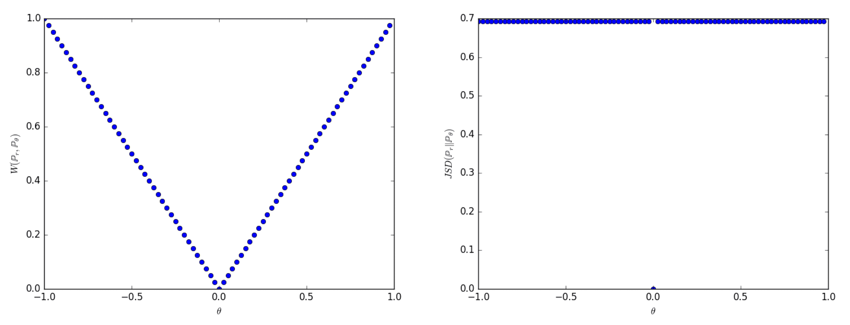
$\mathbf{Fig\ 2.}$ Plots of Wasserstein (left) and JS (right) as a function of $\theta$ (source: [2])

Furthermore, this example demonstrates a scenario where we can train a probability distribution over a low-dimensional manifold by applying gradient descent on the Wasserstein distance. This approach is not viable with other distances and divergences due to lack of continuity. Despite the simplicity of this example involving distributions with disjoint supports, the same outcome holds true when the supports have a non-empty intersection contained within a set of measure zero [3].

The continuity and almost everywhere differentiability of the Wasserstein distance allow us to train the critic $f_w$ until it reaches optimality. In contrast, with the Jensen-Shannon (JS) divergence used in traditional GANs, as the discriminator improves, the gradients become more reliable, but they ultimately tend toward $0$ due to local saturation of the JS divergence, resulting in vanishing gradients, as shown in the theorem by [1]:

$\color{red}{\mathbf{Theorem.}}$ Vanishing gradients on the generator of minimax GAN
Let $G_\theta : \mathcal{Z} \to \mathcal{X}$ be a differentiable function that induces a distribution $\mathbb{P}_g$. Let $\mathbb{P}_r$ be the real data distribution. Let $D: \chi \to [0, 1]$ be a differentiable discriminator and $D^*: \chi \to [0, 1]$ be an optimal discriminator. If the following assumptions hold:

1. Two distributions $\mathbb{P}_r$ and $\mathbb{P}_g$ have support contained on two disjoint compact subsets $\mathcal{M}$ and $\mathcal{P}$ respectively;
2. Two distributions $\mathbb{P}_r$ and $\mathbb{P}_g$ are continuous in their respective manifolds $\mathcal{M}$ and $\mathcal{P}$ that don’t perfectly align and don’t have full dimension, meaning that if there is a set $A$ with measure $0$ in $\mathcal{M}$, then $\mathbb{P}_r (A) = 0$ (and analogously for $\mathbb{P}_g$);
3. $\sup _{x \in \mathcal{X}} | (D - D^*) (x) | + \lVert \nabla (D - D^*) (x) \rVert_2 < \varepsilon$ and $\mathbb{E}_{z \sim p} [\lVert J_\theta G_\theta (z) \rVert_2^2] \leq M^2$;

then $$ \begin{aligned} \left\|\nabla_\theta \mathbb{E}_{z \sim p(z)}\left[\log \left(1-D\left(g_\theta(z)\right)\right)\right]\right\|_2<M \frac{\epsilon}{1-\epsilon} \end{aligned} $$ which implies $$ \begin{aligned} \lim _{\left\|D-D^*\right\| \rightarrow 0} \nabla_\theta \mathbb{E}_{z \sim p(z)}\left[\log \left(1-D\left(g_\theta(z)\right)\right)\right]=0 \end{aligned} $$

$\mathbf{Proof.}$

Since it requires many theorems to prove, I will address them in another post and skip the details here.

\[\tag*{$\blacksquare$}\]

Also the following figure shows an experimental proof for this, where GAN discriminator and WGAN critic are trained until their optimality when learning to differentiate two Gaussians.

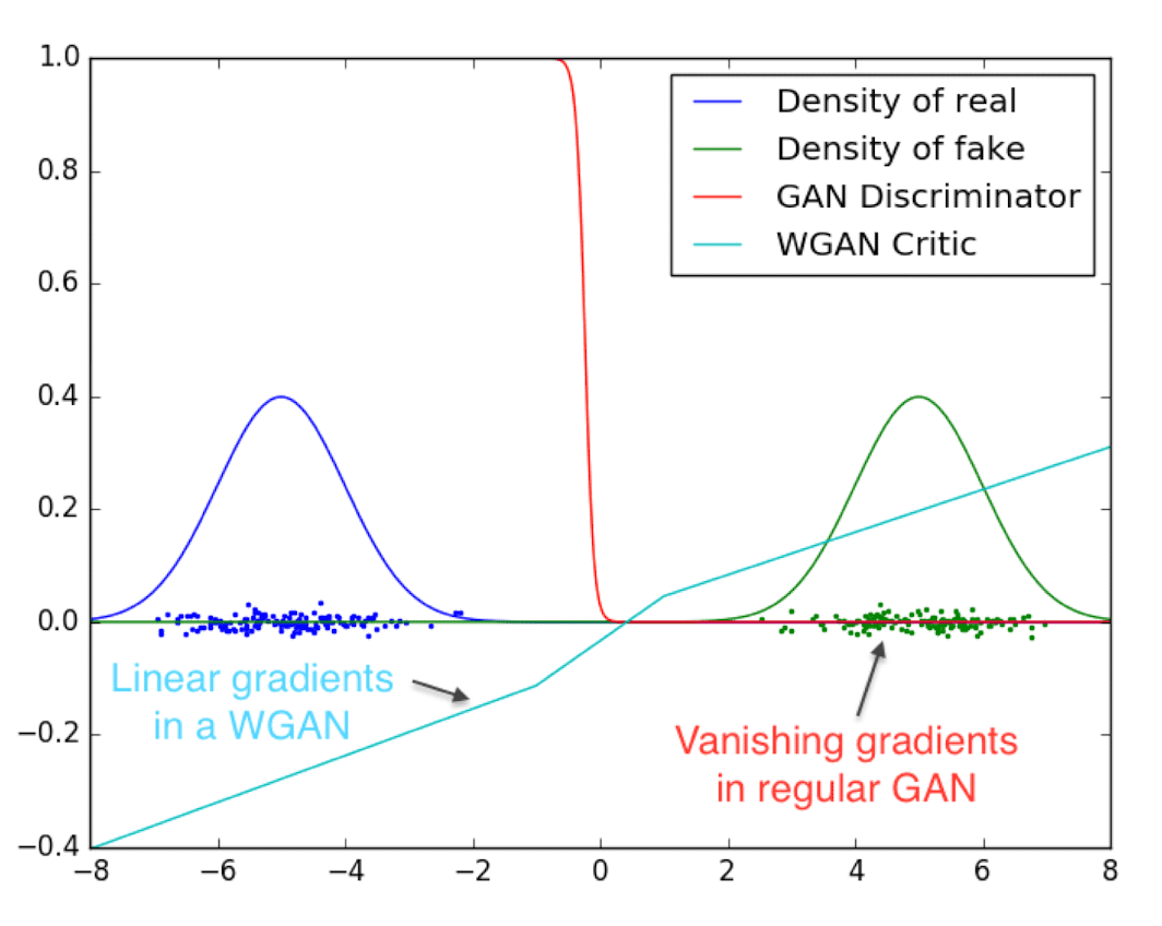
$\mathbf{Fig\ 3.}$ The discriminator of minimax GAN experiences vanishing gradients.
In contrast, WGAN critic produces clean gradients across the entire space. (source: [2])

Impact on convergence

$\color{red}{\mathbf{Theorem.}}$ Relative strength of topology
Let $\mu$ be a distribution on a compact space $\chi$ and $(\mu_n)_{n \in \mathbb{N}}$ be a sequence of distributions on $\chi$. Then, the topology induced by KL is the strongest, followed by JS and TV, and that of Wasserstein distance is the weakest. In other words,

1. The following are equivalent:
   • $\text{TV}(\mu_n, \mu) \to 0$
   • $\text{JS}(\mu_n, \mu) \to 0$
2. The following are equivalent:
   • $W(\mu_n, \mu) \to 0$
   • $\mu_n$ converges to $\mu$ in distribution for random variables.
3. $\text{KL}(\mu_n \Vert \mu) \to 0$ or $\text{KL}(\mu \Vert \mu_n) \to 0$ imply the statements in (1).
4. The statements in (1) imply the statements in (2).

$\mathbf{Proof.}$

(1) $\text{TV}(\mu_n, \mu) \to 0 \Rightarrow \text{JS}(\mu_n, \mu) \to 0$
Let’s denote $\frac{1}{2} \mu_n + \frac{1}{2} \mu$ by $\mu_m$, where $m$ depends on $n$. First, we show that $\text{TV}(\mu_m, \mu_n) \leq \text{TV}(\mu_n, \mu)$. Let $\mu$ be a signed measure and define

\[\begin{aligned} \lVert \mu \rVert_{\text{TV}} = \sup _{A \in \mathcal{B}} | \mu (A) | \end{aligned}\]

where $\mathcal{B}$ is the collection of Borel sets in $\chi$. Then

\[\begin{aligned} \text{TV} (\mu_m, \mu_n) & = \lVert \mu_m - \mu_n \rVert_{\text{TV}} \\ & = \frac{1}{2} \lVert \mu - \mu_n \rVert_{\text{TV}} \\ & = \frac{1}{2} \text{TV}(\mu, \mu_n) \leq \text{TV}(\mu, \mu_n). \end{aligned}\]

Next, let $f_n = d\mu_n / d\mu_m$ be the Radon-Nikodym derivative. (Note that $\mu_n \ll \mu_m$.) For \(A = \{ f_n > 3 \}\) we obtain

\[\begin{aligned} \mu_n (A) = \int_A f_n \; d \mu_m \geq 3 \mu_m (A) \end{aligned}\]

Also, by definition of $\mu_m$, for any borel set $B$ we have $\mu_n (B) \leq 2 \mu_m (B)$. Since $f_n$ is Borel measurable, we may set $B = A$. Thus $\mu_m (A) = 0$. Hence $f_n$ is bounded by $3$ $\mu_m$-a.e.

Let any $\varepsilon > 0$ be given and \(A_n = \{ f_n > 1 + \varepsilon \}\). Then

\[\begin{aligned} \varepsilon \mu_m (A) & < \mu_n (A_n) - \mu_m (A_m) \\ & \leq | \mu_n (A_n) - \mu_m (A_m) | \\ & \leq \text{TV}(\mu_n, \mu_m) \\ & \leq \text{TV}(\mu_n, \mu). \end{aligned}\]

thus $\mu_m(A_n) \leq \text{TV} (\mu_n, \mu) / \varepsilon$. Furhtermore,

\[\begin{aligned} \mu_n (A_n) & \leq \mu_m (A_n) + | \mu_n (A_n) - \mu_m (A_n) | \\ & \leq \frac{1}{\varepsilon} \text{TV}(\mu_n, \mu) + \text{TV}(\mu_n, \mu_m) \\ & \leq \frac{1}{\varepsilon} \text{TV}(\mu_n, \mu) + \text{TV}(\mu_n, \mu) \\ & \leq \left(\frac{1}{\varepsilon} + 1 \right) \text{TV}(\mu_n, \mu) \end{aligned}\]

Finally, we now can see that

\[\begin{aligned} \text{KL} (\mu_n \Vert \mu_m) & = \int \log f_n \; d\mu_n \\ & \leq \log(1 + \varepsilon) + \int_{A_n} \log f_n \; d\mu_n \\ & \leq \log(1 + \varepsilon) + \log 3 \mu_n (A_n) \\ & \leq \log(1 + \varepsilon) + \log 3 \left( \frac{1}{\varepsilon} + 1 \right) \text{TV}(\mu_n, \mu) \end{aligned}\]

By taking limsup we get

\[\begin{aligned} 0 \leq \text{ lim sup} _n \text{KL} (\mu_n \Vert \mu_m) \leq \log(1 + \varepsilon) \end{aligned}\]

for all $\varepsilon > 0$, hence $\text{KL} (\mu_n \Vert \mu_m) \to 0$. Similarly, we can obtain $\text{KL} (\mu \Vert \mu_m) \to 0$. Finally, we conclude

\[\begin{aligned} \text{JS}(\mu_n, \mu) \to 0. \end{aligned}\]

$\text{JS}(\mu_n, \mu) \to 0 \Rightarrow \text{TV}(\mu_n, \mu) \to 0$

Recall the Pinsker’s inequalities:

\[\begin{aligned} \text{TV}(\mu, \nu) \leq \sqrt{\frac{1}{2} \text{KL}(\mu \Vert \nu)}. \end{aligned}\]

Thus, by triangular inequality and Pinsker’s inequalities:

\[\begin{aligned} \text{TV}(\mu_n, \mu) & \leq \text{TV}(\mu_n, \mu_m) + \text{TV}(\mu_m, \mu) \\ & \leq \sqrt{\frac{1}{2} \text{KL}(\mu_n \Vert \mu_m)} + \sqrt{\frac{1}{2} \text{KL}(\mu \Vert \mu_m)} \\ & \leq 2 \sqrt{\text{JS}(\mu_n, \mu)} \to 0. \end{aligned}\]

(2) See Ch 6. of [4].

(3) It is trivial by Pinsker’s inequality.

(4) See appendix A of [2].

\[\tag*{$\blacksquare$}\]

Well-definedness

From Example 1, we observe that Wasserstein distance is viable even on the low-dimensional manifold while others are not. The Wasserstein metric is the only one that offers a smooth gradient and it is highly advantageous for ensuring a stable training through gradient descents.

Also, the following theorem shows the existence of solution and the tractability of gradient for optimization problem:

$\color{red}{\mathbf{Theorem.}}$ Well-definedness of optimization problem
Let $\mathbb{P}_r$ be any distribution. Let $\mathbb{P}_{\theta}$ be the distribution of $G_\theta (Z)$ with a random variable $Z$ with its density $p$, and $G_\theta (Z)$ satisfies the regularity assumption. Then, there exists a solution $f: \chi \to \mathbb{R}$ to the problem $$ \begin{aligned} \max _{\lVert f \rVert_L \leq 1} \mathbb{E}_{X \sim \mathbb{P}_r} [f(X)] - \mathbb{E}_{X \sim \mathbb{P}_\theta} [f(X)] \end{aligned} $$ and we have $$ \begin{aligned} \nabla_{\theta} W(\mathbb{P}_r, \mathbb{P}_\theta) = - \mathbb{E}_{Z \sim p} [\nabla_{\theta} f(G_\theta (Z)) ] \end{aligned} $$ when both terms are well-defined.

$\mathbf{Proof.}$

Step 1.

Denote

\[\begin{aligned} C_b (\chi) = \{f : \chi \to \mathbb{R}, f \text{ is continuous and bounded } \} \end{aligned}\]

Note that if $f \in C_b(\chi)$, we can define its $L^\infty$ norm. Also we will use the following facts for the proof:

1. Every compact metric space is bounded;
2. Every compact metric space is complete;

Therefore if the Lipschitz norm of a function $f$ with its domain $\chi$ is bounded, then $f$ is Lipschitz function thus bounded on a bounded domain.

Define

\[\begin{aligned} V(\widetilde{f}, \theta) & = \mathbb{E}_{X \sim \mathbb{P}_r} [\widetilde{f} (X)] - \mathbb{E}_{X \sim \mathbb{P}_\theta} [\widetilde{f} (X)] \\ & = \mathbb{E}_{X \sim \mathbb{P}_r} [\widetilde{f} (X)] - \mathbb{E}_{Z \sim p} [\widetilde{f} (G_\theta (Z))] \end{aligned}\]

where $\widetilde{f}$ lies in \(\mathcal{F} = \{ \widetilde{f} : \chi \to \mathbb{R}, \widetilde{f} \in C_b (\chi), \lVert \widetilde{f} \rVert_L \leq 1 \}\) and $\theta \in \mathbb{R}^d$. Since $\chi$ is compact metric space, from the fact that every compact metric space is complete, $\chi$ is complete. Then by Kantorovich-Rubinstein theorem, there exists an $f \in \mathcal{F}$ that attains the supremum:

\[\begin{aligned} W (\mathcal{P}_r, \mathcal{P}_\theta) = \sup _{\widetilde{f} \in \mathcal{F}} V(\widetilde{f}, \theta) = V(f, \theta). \end{aligned}\]

Thus, the following set is not an emptyset for each $\theta$:

\[\begin{aligned} X^* (\theta) = \left\{ f \in \mathcal{F} : V(f, \theta) = W (\mathcal{P}_r, \mathcal{P}_\theta) \right\} \end{aligned}\]

By the envelope theorem, we have

\[\begin{aligned} \nabla_{\theta} W(\mathbb{P}_r, \mathbb{P}_\theta) = \nabla_{\theta} V (f, \theta) \end{aligned}\]

for any $f \in X^* (\theta)$ when both terms are well-defined. Let $f \in X^* (\theta)$. Then we get

\[\begin{aligned} \nabla_{\theta} W(\mathbb{P}_r, \mathbb{P}_\theta) & = \nabla_{\theta} V (f, \theta) \\ & = \nabla_{\theta} [\mathbb{E}_{x \sim P_r} [f(x)] - \mathbb{E}_{z \sim p} [f(G_\theta(z))]] \\ & = - \nabla_{\theta} \mathbb{E}_{z \sim p} [f(G_\theta(z))] \end{aligned}\]

under the condition that the first and last terms are well-defined.

Step 2.

Now we will see that

\[\begin{aligned} - \nabla_{\theta} \mathbb{E}_{z \sim p} [f(G_\theta(z))] = - \mathbb{E}_{z \sim p} [\nabla_{\theta} f(G_\theta(z))] \end{aligned}\]

when the RHS is defined. Since $f \in \mathcal{F}$, we know that it is $1$-Lipschitz continuous. Furthermore, $G$ is locally Lipschitz as a function of $(\theta, z)$ by regularity assumption. Therefore, $f(G_\theta(z))$ is locally Lipschitz on $(\theta, z)$ with constants $L(\theta, z)$ (the same ones as $g$). Also, by Radamacher’s Theorem, it is differentiable almost everywhere for $(\theta, z)$ jointly. Thus the set

\[\begin{aligned} A = \{ (\theta, z) : f \cdot G \text{ is not differentiable }\} \end{aligned}\]

has measure $0$. By Fubini’s Thoerem, this implies that for almost every $\theta$ the section \(A_\theta = \{ z: (\theta, z) \in A \}\) has measure $0$, too. Fix a $\theta_0$ such that the measure of \(A_{\theta_0}\) is null and also \(- \mathbb{E}_{z \sim p} [\nabla_{\theta} f(G_\theta(z))]\) is well-defined for $\theta_0$. Hence for this $\theta_0$ we have well-defined \(\nabla_{\theta} f(G_\theta (\theta)) \|_{\theta_0}\) for almost any $z$ and by the regularity assumption

\[\begin{aligned} \mathbb{E}_{z \sim p} [\lVert \nabla_{\theta} f(G_\theta (\theta)) |_{\theta_0} \rVert] \leq \mathbb{E}_{z \sim p} [L(\theta_0, z)] < \infty. \end{aligned}\]

Now we can see

\[\begin{aligned} & \frac{\mathbb{E}_{z \sim p}\left[f\left(G_\theta(z)\right)\right]-\mathbb{E}_{z \sim p}\left[f\left(G_{\theta_0}(z)\right)\right]-\left\langle\left(\theta-\theta_0\right), \mathbb{E}_{z \sim p}\left[\left.\nabla_\theta f\left(G_\theta(z)\right)\right|_{\theta_0}\right]\right\rangle}{\left\|\theta-\theta_0\right\|} \\ = \; & \mathbb{E}_{z \sim p}\left[\frac{f\left(G_\theta(z)\right)-f\left(G_{\theta_0}(z)\right)-\left\langle\left(\theta-\theta_0\right),\left.\nabla_\theta f\left(G_\theta(z)\right)\right|_{\theta_0}\right\rangle}{\left\|\theta-\theta_0\right\|}\right] \end{aligned}\]

By differentiability, the term inside the integral converges to $0$ as $\theta \to \theta_0$ for almost every $z$. Furthermore,

\[\begin{aligned} & \left\|\frac{f\left(G_\theta(z)\right)-f\left(G_{\theta_0}(z)\right)-\left\langle\left(\theta-\theta_0\right),\left.\nabla_\theta f\left(G_\theta(z)\right)\right|_{\theta_0}\right\rangle}{\left\|\theta-\theta_0\right\|}\right\| \\ \leq \; & \frac{\left\|\theta-\theta_0\right\| L\left(\theta_0, z\right)+\left\|\theta-\theta_0\right\|\left\|\left.\nabla_\theta f\left(G_\theta(z)\right)\right|_{\theta_0}\right\|}{\left\|\theta-\theta_0\right\|} \leq 2L(\theta_0, z) \end{aligned}\]

and since $\mathbb{E}_{z \sim p} [2L(\theta_0, z)] < \infty$ by the regularity assumption, by dominated convergence

\[\begin{aligned} \nabla_{\theta} \mathbb{E}_{z \sim p} [f(G_\theta (z))] = \mathbb{E}_{z \sim p} [\nabla_{\theta} f(G_\theta (z))] \end{aligned}\]

for almost every $\theta$ and when the RHS is well-defined.

\[\tag*{$\blacksquare$}\]

Reference

[1] Dudley RM. Real Analysis and Probability. 2nd ed. Cambridge: Cambridge University Press; 2002..
[2] Arjovsky, Martin, Soumith Chintala, and Léon Bottou. “Wasserstein Generative Adversarial Networks.” International conference on machine learning. PMLR, 2017.
[3] Martin Arjovsky and Léon Bottou. Towards principled methods for training generative adversarial networks. In International Conference on Learning Representations, 2017.
[4] Villani, Cédric. Optimal transport: old and new. Vol. 338. Berlin: springer, 2009.
[5] Virmaux, Aladin, and Kevin Scaman. “Lipschitz regularity of deep neural networks: analysis and efficient estimation.” NeurIPS (2018).