[Generative Model] Diffusion Transformer (DiT)

Transformers have exhibited exceptional scaling properties across a plethora of domains, such as language modeling and computer vision. In light of the outstanding success of Transformers, Peebles et al. 2023 proposed a novel class of diffusion models founded on Transformers, called Diffusion Transformer (DiT).

$\mathbf{Fig\ 1.}$ The Diffusion Transformer (DiT) architecture (Peebles et al., 2023)

Architectural Design

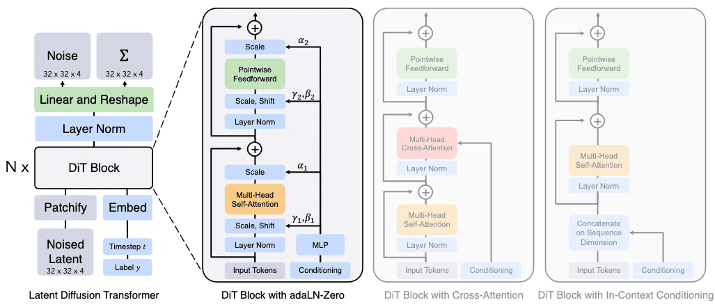
Diffusion Transformer (DiT) is Latent Diffusion Model (LDM) based on the Vision Transformer (ViT) architecture, which operates on sequences of patches, instead of U-Net.

Patchify

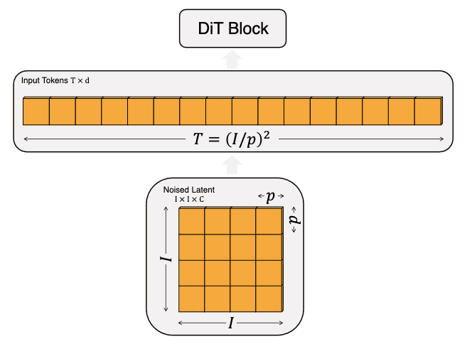
Given patch size $p \times p$, a spatial representation $z$ (the noised latent from the VAE encoder) with dimensions $I \times I \times C$ is patchified into a sequence of length $T = (I/p)^2$ with a hidden dimension $d$. It is important to note that a smaller patch size $p$ leads to a longer sequence length, consequently increasing the number of Gflops.

$\mathbf{Fig\ 2.}$ Input specifications for DiT (Peebles et al., 2023)

DiT Block

Following patchification, ViT positional embeddings are applied to all input tokens, which are then processed by a sequence of transformer blocks. To incorporate conditional information for diffusion generation such as noise timesteps $t$, class labels $c$ and text, DiT adopts a block design with adaptive layer normalization layers as introduced in FiLM.

\[\mathbf{x}^\prime = \gamma \cdot \frac{\mathbf{x} - \mu (\mathbf{x})}{\sigma (\mathbf{x})} + \beta \text{ where } \mathbf{x}, \mathbf{x}^\prime \in \mathbb{R}^d\]

The scaling parameters $\gamma$ and $\beta$ of adaLN are regressed from the sum of the vector embeddings of $t$ and $c$:

\[\gamma = f(\mathbf{z}_{\texttt{embed}}) \quad \beta = h(\mathbf{z}_{\texttt{embed}})\]

where functions $f$ and $h$ are trained and $\mathbf{z}_{\texttt{embed}} = \mathbf{z}_t + \mathbf{z}_c \in \mathbb{R}^d$. Note that the embedding $\mathbf{z}_t$ of $t$ and $\mathbf{z}_c$ of $c$ are processed by two-layer MLPs with SiLU activations:

\[\texttt{SiLU}(x) = x \cdot \texttt{sigmoid}(x) = \frac{x}{1 + e^{-x}}\]

Furthermore, dimension-wise scalings are applied immediately prior to any residual connections within the DiT block, which the parameters $\alpha$ also being regressed.

$\mathbf{Fig\ 3.}$ Adaptive layer norm (adaLN) DiT block (Peebles et al., 2023)

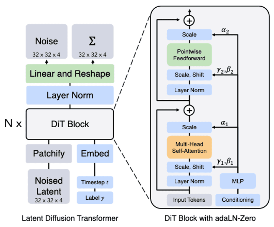
After the final DiT block, the output feature is deocoded into noise prediction $\boldsymbol{\varepsilon}$ and diagonal covariance prediction $\boldsymbol{\Sigma}$ that have shape equal to the original spatial input. Specifically, the linear layer decodes each token into $p \times p \times 2C$ tensor, where $C$ is the number of channels in the spatial input to DiT, and this tensor is rearragned to the original spatial shape to get the predicted noise and covariance.

Model size

Similar to ViT, DiT can be categorized into $4$ configurations:

• DiT-S
• DiT-B
• DiT-L
• DiT-XL

based on the number of layer $N$, the hidden size $d$ and the number of attention heads $H$.

$\mathbf{Fig\ 4.}$ Details of DiT models (Peebles et al., 2023)

Scaling DiT

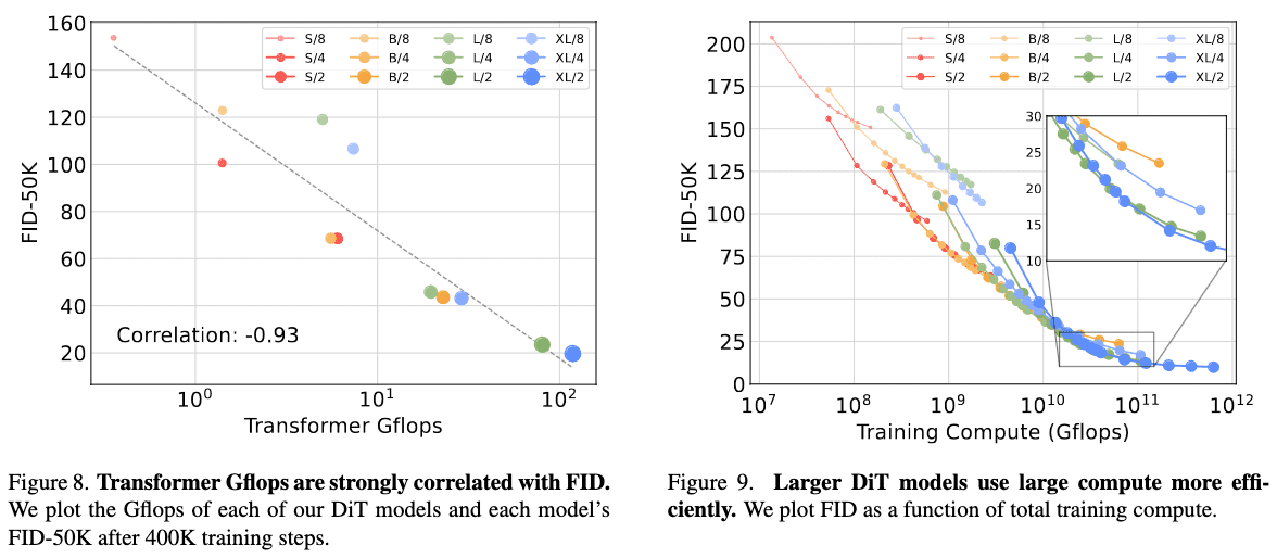
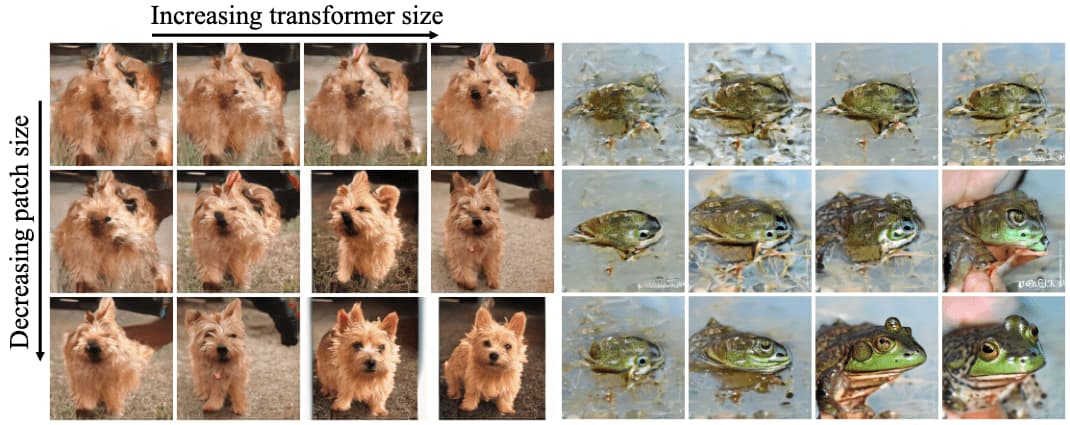
The authors discovered that DiT is highly scalable; augmenting model size and reducing patch size significantly enhance the performance of diffusion models at every stage of training.

$\mathbf{Fig\ 5.}$ Scaling the DiT improves FID at all stages of training (Peebles et al., 2023)

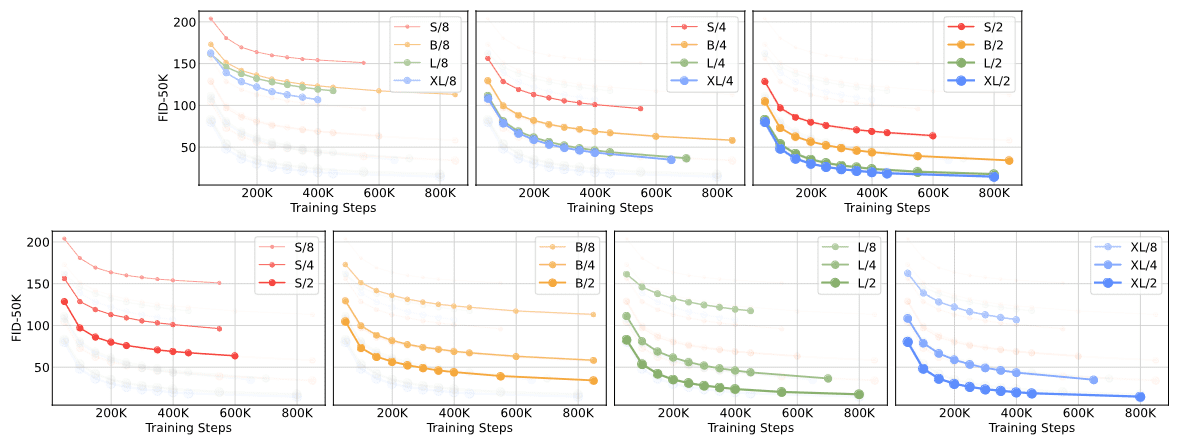
Interestingly, different DiT configurations achieve similar FID scores when their total Gflops are comparable. This implies that parameter counts do not solely determine the performance. Instead, increased model compute is the crucial factor for enhancing DiT models, as evidenced by the strong negative correlation between model Gflops and FID score.

The authors also observed that larger DiT models are more compute-efficient compared to smaller models; the larger models require less training compute to achieve a given FID than smaller models. Here, training compute is estimated by Gflops $\times$ batch size $\times$ training steps $\times 3$, where the factor of $3$ approximates the backward pass as being twice as compute-intensive as the forward pass.

$\mathbf{Fig\ 6.}$ DiT Gflops are critical to improving performance & Larger DiT models are more compute-efficient. (Peebles et al., 2023)

In quantatitve comparison, the authors also observed that scaling both model size and the number of tokens results in substantial improvements in visual quality.

$\mathbf{Fig\ 7.}$ Increasing transformer forward pass Gflops increases sample quality (Peebles et al., 2023)

Comparison to SOTA Diffusions

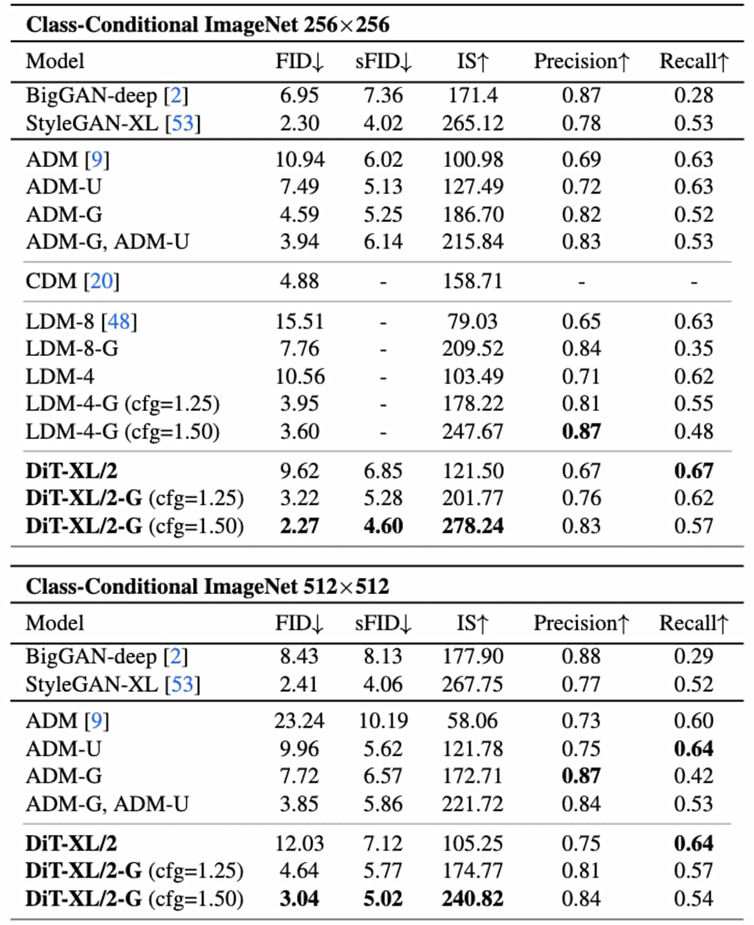
Consequently, DiT with classifier-free guidance outperforms all prior diffusion models in both $256 \times 256$ and $512 \times 512$ resolutions.

$\mathbf{Fig\ 8.}$ Benchmarking class-conditional image generation on ImageNet (Peebles et al., 2023)

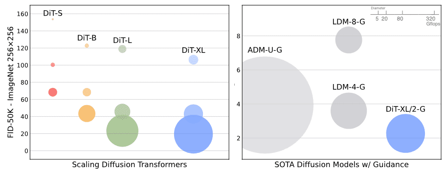
In addition to achieving good FIDs, the DiT model remains compute-efficient compared to other diffusions. The following figure displays the FID plot of DiTs and prior SOTA diffusion models, including classifier-guided diffusion (ADM) and latent diffusion model (LDM). Bubble area in the figure represents the flops of the diffusion model. For example, at $256 \times 256$ resolution, the LDM-4 model is $103$ Gflops, ADM-U is $742$ Gflops and DiT-XL/2 is $119$ Gflops. At $512 \times 512$ resolution, ADM-U requires $2813$ Gflops whereas XL/2 needs only $525$ Gflops.

$\mathbf{Fig\ 9.}$ ImageNet generation with Diffusion Transformers (DiTs) (Peebles et al., 2023)

Reference

[1] Peebles et al., “Scalable Diffusion Models with Transformers”, ICCV 2023 Oral