[Linear Algebra] Definiteness

Definiteness of matrix plays an instrumental role in various areas of mathematics, such as convex optimization. It also even comes a lot in statistics, especially multivariate statistics. And we will see in this post, when the space is extended to high-dimensional space, It can be thought of as defining signs for matrices such as positive/negative numbers.

$\color{blue}{\mathbf{Def.}}$ Quadratic Forms
A quadratic form is a polynomial with terms all of degree two. For example,

\[\begin{aligned} 4x^2 + 2xy - 3y^2 \end{aligned}\]

$\color{cyan}{\mathbf{Remark.}}$

1. Any $n \times n$ matrix $A$ can determine a quadratic form $q_A$:
   $$ \begin{aligned} q_A (x_1, \dots, x_n) = \sum_{i=1}^n \sum_{j=1}^n a_{ij} x_i x_j = \mathbf{x}^\top A \mathbf{x} \end{aligned} $$
2. We can just assume that $A$ in $q_A$ is always symmetric, because for any $n \times n$ matrix $A$ in the corresponding quadratic form $q_A$, there exists a symmetric $B \in \mathbb{R}^{n \times n}$ such that $$ \begin{aligned} \mathbf{x}^\top B \mathbf{x} = \mathbf{x}^\top A \mathbf{x} \end{aligned} $$
   For example, $B = \frac{1}{2} (A + A^\top)$.

---

Definite Matrix

$\color{blue}{\mathbf{Def.}}$ Definiteness of symmetric matrix
Let $A \in \mathbb{R}^{n \times n}$ be a symmetric matrix.

1. $A$ is positive definite (p.d.) if for all non-zero vectors $\mathbf{x}\in \mathbb{R}^n$,
   $$ \begin{aligned} \mathbf{x}^\top A \mathbf{x} > 0 \end{aligned} $$
2. $A$ is positive semi-definite (p.s.d.) if for all non-zero vectors $\mathbf{x}\in \mathbb{R}^n$,
   $$ \begin{aligned} \mathbf{x}^\top A \mathbf{x} \geq 0 \end{aligned} $$
3. $A$ is negative definite (n.d.) if for all non-zero vectors $\mathbf{x}\in \mathbb{R}^n$,
   $$ \begin{aligned} \mathbf{x}^\top A \mathbf{x} < 0 \end{aligned} $$
4. $A$ is negative semi definite (n.s.d.) if for all non-zero vectors $\mathbf{x}\in \mathbb{R}^n$,
   $$ \begin{aligned} \mathbf{x}^\top A \mathbf{x} \leq 0 \end{aligned} $$
5. $A$ is indefinite if $A$ is none of above.

Equivalent Definitions

Recall that every symmetric matrix can be decomposed to eigenvalue decomposition. Hence, we can easily derive the equivalent definitions of definiteness with eigenvalues:

$\color{red}{\mathbf{Thm\ 1.}}$ Definitions with Eigenvalues
Let $A \in \mathbb{R}^{n \times n}$ be a symmetric matrix.

1. $A$ is positive definite (p.d.) if and only if all of its eigenvalues are positive.
2. $A$ is positive semi-definite (p.s.d.) if and only if all of its eigenvalues are non-negative.
3. $A$ is negative definite (n.d.) if and only if all of its eigenvalues are negative.
4. $A$ is negative semi-definite (n.s.d.) if and only if all of its eigenvalues are non-positive.
5. $A$ is indefinite if and only if it has both positive and negative eigenvalues.

The forward direction is trivial. If $A$ is symmetric (let $A = Q^\top \Lambda Q$ be an eigenvalue decomposition of $A$) and its all of eigenvalues are positive, for any non-zero vector $\mathbf{x} \in \mathbb{R}^n$

\[\begin{aligned} \mathbf{x}^\top A \mathbf{x} = \mathbf{x}^\top Q^\top \Lambda Q \mathbf{x} = (Q \mathbf{x})^\top \Lambda (Q \mathbf{x}) = \mathbf{y}^\top \Lambda \mathbf{y} = \sum_{i=1}^n \lambda_i y_i^2 > 0 \end{aligned}\]

as $\mathbf{y} = Q \mathbf{x}$ is non-zero vector since $Q$ is invertible and $\mathbf{x}$ is non-zero. Other definitions can be proved in analogous ways.

And it leads to relationship with determinant $\text{det}(A) = \prod_{i=1}^n \lambda_i$:

$\color{blue}{\mathbf{Corollary.}}$ Determinant of definite matrix
Let $A \in \mathbb{R}^{n \times n}$ be a symmetric matrix.

1. If $A$ is positive definite, then $\color{blue}{\text{det}(A) > 0}$.
2. If $A$ is positive semi-definite, then $\color{blue}{\text{det}(A) \geq 0}$.

Intuition: Sign of matrix

As it was mentioned, we can understand the definiteness of matrix as a sign of matrix intuitively.

If a symmetric matrix $A$ is positive definite or positive semi-definite, a linear transformation $T(\mathbf{x}) = A \mathbf{x}$ induced by $A$ does not “flip” the vector $\mathbf{x}$ about the origin; it preserves the direction of original vector $\mathbf{x}$. In terms of the cosine angle between $\mathbf{x}$ and $A \mathbf{x}$, it preserves the angle within -90° ~ 90°:

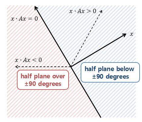
$\mathbf{Fig\ 1.}$ Linear transformation induced by definite matrix (source: Angelo's Math Notes)

Otherwise, negative (semi) definite matrix will flip the direction of vector. These geometric interpretation coincides with preservation or flip of sign of real numbers by multiplication.

Let’s further delve into comparisons with real numbers. It is trivial that if any real number $x \in \mathbb{R}$ is non-negative, i.e. $x \geq 0$, there exists a root of $x$ $\sqrt{x} \in \mathbb{R}$ in real line. And conversely if $\sqrt{x} \in \mathbb{R}$, it is clear that $x \geq 0$. Equivalently, there is a similar theorem with positive semi-definite matrix:

$\color{red}{\mathbf{Thm\ 3.}}$
Let $A$ be $n \times n$ symmetrix matrix. $A$ is positive semi-definite if any only if $A$ is Gram matrix; there exists a matrix $Q$ where

\[\begin{aligned} A = Q^\top Q \end{aligned}\]

$\color{red}{\mathbf{Proof.}}$

If $A$ is positive semi-definite, all eigenvalues of $A$ is non-negative. Hence,

\[\begin{aligned} A = Q^\top \Lambda Q = Q^\top \Lambda^{1/2} \Lambda^{1/2} Q = (\Lambda^{1/2} Q)^\top \Lambda^{1/2} Q = M^\top M. \end{aligned}\]

Conversely, if $A = Q^\top Q$ for some matrix $Q$, for any non-zero vector $\mathbf{x} \in \mathbb{R}^n$,

\[\begin{aligned} \mathbf{x}^\top A \mathbf{x} = (Q \mathbf{x})^\top (Q \mathbf{x}) = \| Q \mathbf{x} \|_2^2 \geq 0 \quad \blacksquare \end{aligned}\]

In another instance, let’s envision the invertibility of real number. Let $x \in \mathbb{R}$ and $x \geq 0$. If $x^{-1} = \frac{1}{x} \in (- \infty, \infty)$, it is clear that $x > 0$. And if $x \in \mathbb{R}$ and $x > 0$, then we also know that $x^{-1} \in (- \infty, \infty)$ too. Indeed, these basic fact corresponds to the following theorem of definite matrix:

$\color{red}{\mathbf{Thm\ 4.}}$
Let $A$ be $n \times n$ symmetrix matrix.

1. If $A$ is positive definite or negative definite, then $A$ is invertible.
2. If $A$ is invertible and positive semi-definite (or negative semi-definite), then $A$ is positive definite (or negative definite)

$\color{red}{\mathbf{Proof.}}$

Let $A = Q^\top \Lambda Q$ be an eigenvalue decomposition of $A$. Recall that $\text{rank}(A) = \text{rank}(\Lambda)$.

1. If $A$ is p.d., all eigenvalues are positive, i.e., non-zero. Hence, it implies a diagonal matrix $\Lambda$, which diagonal entries are eigenvalues of $A$, is a full rank. So does negative definite case.
2. If $A$ is full rank, every eigenvalue of $A$ should be non-zero. Since all eigenvalues of $A$ are non-negative, every eigenvalue should be positive, i.e. $A$ is positive definite. So does negative semi-definite case. $\blacksquare$

Hence, we often denote the definiteness of matrix with inequality:

1. $A$ is positive definite $\Leftrightarrow \; A \color{blue}{>} 0$
2. $A$ is positive semi-definite $\Leftrightarrow \; A \color{blue}{\geq} 0$
3. $A$ is negative definite $\Leftrightarrow \; A \color{blue}{<} 0$
4. $A$ is negative semi-definite $\Leftrightarrow \; A \color{blue}{\leq} 0$

Application: Convexity

In basic calculus, we remember that the second derivative $f^{\prime \prime} (x)$ of function $f: \mathbb{R} \to \mathbb{R}$ telss us the rate at which the derivative changes, so that it indicates the convexity of function. If $f^{\prime \prime}(x) > 0$ for all $x \in \mathbb{R}$, then $f$ is a convex function and in $f^{\prime \prime}(x) < 0$ case $f$ is a concave function:

$\mathbf{Fig\ 2.}$ Second derivative and convexity

If the dimension of function is extended to high-dimensional case $f: \mathbb{R}^n \to \mathbb{R}$, the second derivative of function is also generalized to Hessian matrix:

\[\begin{aligned} \mathbf{H}_f = \nabla^2 f = \left[\begin{array}{cccc} \frac{\partial^2 f}{\partial x_1^2} & \frac{\partial^2 f}{\partial x_1 \partial x_2} & \cdots & \frac{\partial^2 f}{\partial x_1 \partial x_n} \\ \frac{\partial^2 f}{\partial x_2 \partial x_1} & \frac{\partial^2 f}{\partial x_2^2} & \cdots & \frac{\partial^2 f}{\partial x_2 \partial x_n} \\ \vdots & \vdots & \ddots & \vdots \\ \frac{\partial^2 f}{\partial x_n \partial x_1} & \frac{\partial^2 f}{\partial x_n \partial x_2} & \cdots & \frac{\partial^2 f}{\partial x_n^2} \end{array}\right] \end{aligned}\]

i.e. \((\mathbf{H}_f)_{ij} = \left( \frac{\partial^2 f}{\partial x_i \partial x_j}\right)\). And as we expect, the convexity of high-dimensional function is also determined by definiteness of matrix. If $\nabla^2 f > 0$, $f$ is convex, and if $\nabla^2 f < 0$, then $f$ is concave:

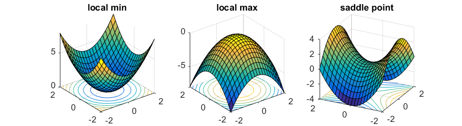
$\mathbf{Fig\ 3.}$ Hessian matrix and convexity

https://gregorygundersen.com/blog/2022/02/27/positive-definite/

Reference

[1] Contemporary Linear Algebra, Howard Anton, Robert C. Busby
[2] Wikipedia, Definite matrix