
[ML] Regression Model - Part I

Linear Regression Model
Let’s denote data by $(\mathbf{x_i} , y_i) = (x_{i1}, \cdots, x_{ik}, y_i)$, $i = 1, 2, \cdots, n$ for $n > k$ and linear regression model by $y_i = \beta_0 + x_{i1} \beta_1 + \cdots + x_{ik} \beta_k + \varepsilon_i = \beta_0 + \sum_{j=1}^k x_{ij} \beta_j + \varepsilon_i$
In matrix form, we have $\mathbf{y} = \boldsymbol{X \beta} + \boldsymbol{\epsilon}$ where
Then our objective is to minimize
\[\begin{aligned} \sum_{i=1}^n \varepsilon_{i}^2 = \sum_{i=1}^n \left[ y_i - (\beta_0 + \sum_{j=1}^k x_{ij} \beta_j) \right]^2 \end{aligned}\]which is equivalent to minimize $f(\boldsymbol{\beta}) := || \mathbf{y} - \boldsymbol{X \beta} ||^2 = (\mathbf{y} - \boldsymbol{X \beta})^\top (\mathbf{y} - \boldsymbol{X \beta}).$
The Analytic Solution: The Normal Equation
By simple calculus, we can obtain the gradient of this error term as:
From $\nabla_{\boldsymbol{\beta}} f(\mathbf{\beta}) = 0$, we get the optimal value of $\boldsymbol{\beta}$, which is equivalent to the least square estimates $\widehat{\boldsymbol{\beta}}$, given by
This equation is known as the normal equation .
But, solving the equation includes computing the inverse of a matrix of $(D + 1) \times (D + 1)$ shape. And, inversing this matrix typically takes $O(D^{2.4})$ to $O(D^3)$ depending on the implementation of the underlying numerical algorithm. This means the computation increases cubically in terms of the number of features, which is very expensive.
Gradient Descent
The object is to find a linear line that explains the dataset well. Then, how can we choose the best line?
First, we consider an objective function:
Objective function : In general, the objective function is the one we optimize, i.e., whose value we want to either minimize or maximize.
Cost function : measures the model’s error on a group of objects, whereas the loss function deals with a single data instance.
Loss function : quantifies how much a model $f$‘s prediction $\boldsymbol{\hat{y} \equiv f(\mathbf{x})}$ deviates from the ground truth $\boldsymbol{y \equiv y(\mathbf{x})}$ for one particular object $\mathbf{x}$. [3]
After setting the objective function, we use gradient descent algorithm to mininize that criterion. The general idea is to tweak the parameters iteratively in order to minimize a cost function. We use the gradient of the cost function to decide the direction of the parameter update. So, gradient descent is applicable to training any model as long as the gradient of the cost function with regard to the parameter is computable. (i.e., to all differentiable cost functions.)
The pseudocode of algorithm is outlined below:
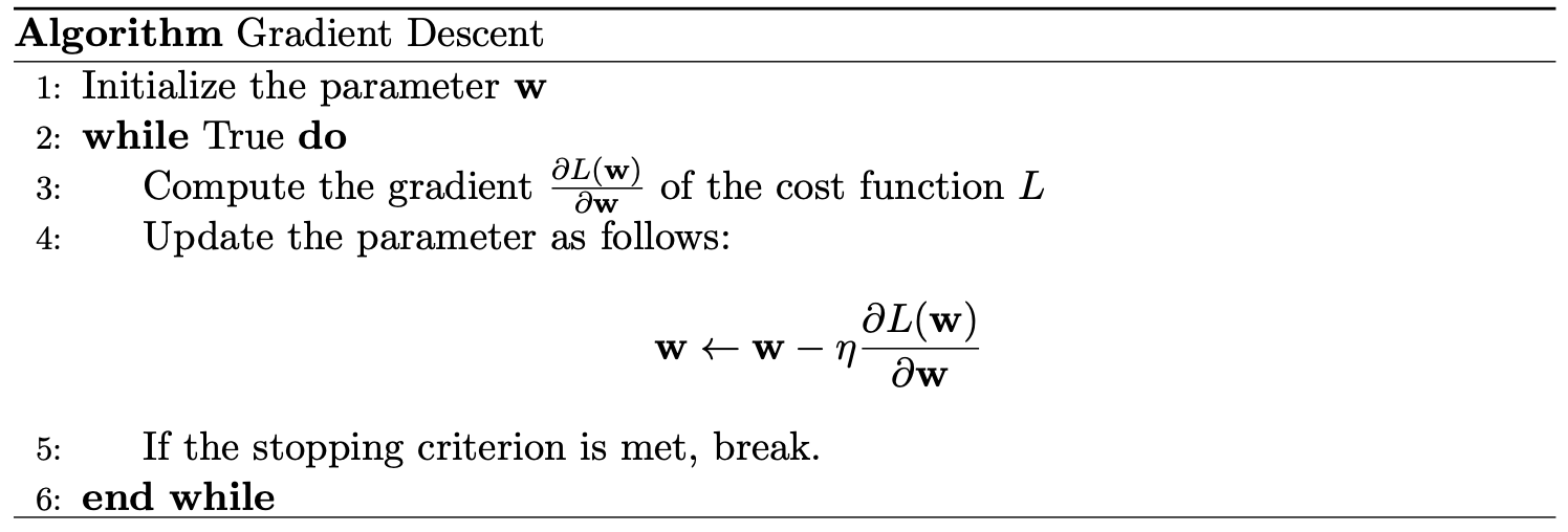
Here, $\eta$ is the learning rate (or step size), a hyperparameter that controls how much move to the direction of the gradient. And learning rate is usually the most important hyperparameter in training a model by gradient descent, especially for neural networks.

And stopping criterion can be anything that met needs of the user. For example, we may stop the algorithm if it doesn’t improve model, in other words, the validation loss doesn’t decrease anymore:

This kind of stopping criterion is referred to as early stopping. Or, the norm of the gradient is near $0$:

Stochastic Gradient Descent
Gradient of the loss function is usually the sum of the gradients of all datapoints. For instance, in case of MSE of linear regression,
\[\begin{aligned} \frac{\partial L(\mathbf{w}, b)}{\partial \mathbf{w}} = \frac{1}{N} \sum_{i=1}^N (\mathbf{w}^\top \mathbf{x}^{(i)} + b - \mathbf{y}^{(i)}) \cdot x^{(i)} \end{aligned}\]And remember that gradient descent is an iterative method requiring to compute the gradients until it converges. Hence it could be one million iterations, or even more! The stochastic gradient descent estimates the gradient using a small mini-batch $\mathcal{M}$ instead of the full dataset $\mathcal{D}$.
Here, $I(\mathcal{M})$ contains the indices of $| \mathcal{M} |$ datapoints which are uniformly-randomly sampled from $1, \cdots, N$. $| \mathcal{M} |$ is usually much smaller than $N$, for example we can use $| \mathcal{M} | = 100$ when $N$ is one million. Since it can make progress with each data sample, so it often has faster convergence than the gradient descent algorithm. Each data sample is randomly selected from which the name stochastic comes.
$\mathbf{Remark.}$ In some literature, SGD means gradient descent when $| \mathcal{M} | = 1$. And if $1 < | \mathcal{M} | < N$, it is called mini-batch GD. But we usually use the term SGD for all cases $| \mathcal{M} | < N$ interchangeably.
Why SGD works?
The reason why SGD works and converges to optimal point correctly is, the stochastic gradient is an unbiased estimator of the true gradient if the minibatch is uniformly randomly sampled. It can be easily verified from the fact that sample mean is an unbiased estimator of the true mean.
Given a dataset $\mathcal{D}$ of size $N$, the true mean value is
To estimate $\mu^*$, if we make an estimator $f$ by uniformly-randomly sampling a subset $\mathcal{M} \subset \mathcal{D}$ with $| \mathcal{M} | \ll N$, we have
Then, we say that $f$ is an unbiased estimator of the true mean as
\[\begin{aligned} \mathbb{E}_{p(\mathcal{M})} [f(\mathcal{M})] = \mu^* \end{aligned}\]Based on this mathematical background, even SGD is noisy but on average still points to the right direction even if $| \mathcal{M} | = 1$.

Practice
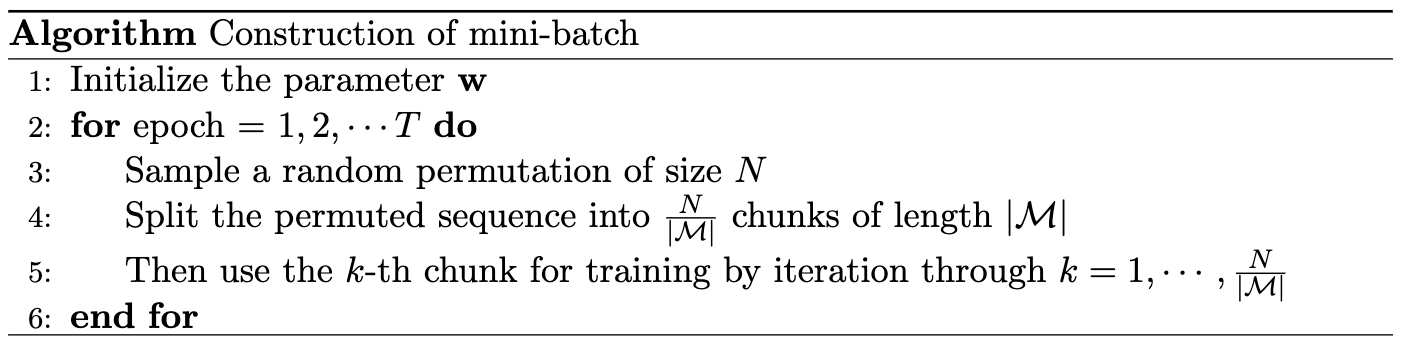
SGD can be simply implemented by random permutation:
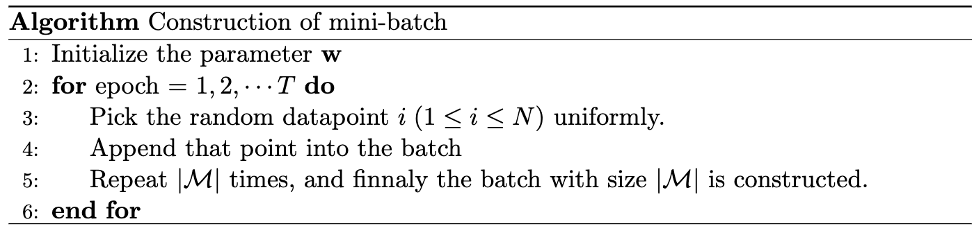
But, if the dataset size $N$ is too big, permutation may be very expensive. We can mitigate this inefficiency by uniform sampling:
SGD and Overfitting
Remember that optimizing too much on training set may result in overfitting. When using SGD, it could be difficult to optimize very accurately due to learning rate and mini-batch noise. Thus, in practice SGD usually provides good generalization performance. But if the step size is too small, a model may overfit.
The Probabilistic Approach
The response of an experiment can be predicted more adequately on the basis of a collection of input variables $Y = \beta_0 + \beta_1 x_1 + \cdots + \beta_k x_k + \varepsilon$ where
- $Y$: random variables
- $x_i$: a set of input (independent) variables
- $\epsilon \sim \mathcal{N}(0, \sigma^2)$: a normal error with unknown $\sigma^2$
Hence it can be interpreted by $Y \sim N(\beta_0 + \beta_1 x_1 + \cdots + \beta_k x_k, \sigma^2)$.
Let $Y_i$ be the response corresponding to the set \(\{ x_{i1}, \cdots, x_{ik} \}\). We now consider the likelihood function of data sample $(y_1, \cdots, y_n)$
where $h_i (\mathbf{\beta}) = \beta_0 + \sum_{j=1}^k \beta_j x_{ij}.$
Then log likelihood function is given by
As a result, to maximize the log likelihood function, it is sufficient to minimize $\sum_{i=1}^n (y_i - h_i (\mathbf{\beta}))^2$, which is identical to $f(\boldsymbol{\beta})$. From this point of view, the least square estimators (LSEs) are also called the maximum likelihood estimators (MLEs), because they give the exactly same solution!
Reference
[1] Christopher M. Bishop, Pattern Recognition and Machine Learning, Springer 2006.
[2] GeÌron, Aureìlien, Hands-on Machine Learning with Scikit-Learn, Keras and TensorFlow: Concepts, Tools, and Techniques to Build Intelligent Systems. 2nd ed., O’Reilly 2019.
[3] Difference Between the Cost, Loss, and the Objective Function
[4] StatQuest with Josh Starmer
Leave a comment