[ML] Probabilistic Linear Regression

Probabilitistic Linear Regression

Motivation

Inevitably, there is an uncertainty in decision making. For example, you make a system predicting stock prices. Suppose that the system predicts that the price of stock A will increase 5% tomorrow. Will you bet all your money? Or, a binary classifier predicting the existence of a cancer says TRUE (exist). Then will you go to a surgery?

These uncertainties raises demand for probabilistic model, instead of deterministic model. Through probabilistic model, we may express the uncertainty over the value of the target variable using a probability distribution.

Construction of a probabilistic model

To construct a probabilistic model, we usually consider the observation (random) noise $\epsilon$ and define

\[\begin{align*} y = f(\mathbf{x}; \mathbf{w}) + \varepsilon \end{align*}\]

For explicit modeling, we need to an assumption about what kind of distribution does the noise $\varepsilon$ follows. One of the most commonly used distribution is Gaussian distribution where leaves the door open for both positive or negative noises and implicit that small noise is more likely than large noise. Then, we can construct a probability

\[\begin{align*} p(y \; | \; \mathbf{x}) = \mathcal{N}(f(\mathbf{x}; \mathbf{w}), \sigma^2) \end{align*}\]

where $f(\mathbf{x}; \mathbf{w}) = \mathbf{x}^\top \mathbf{w}$.

Model Fitting (MLE)

Then, how can we learn this model $\mathcal{N}(f(\mathbf{x}; \mathbf{w}). \sigma^2)$ from the observed data?

In statistics, this point estimation problem involves the use of sample data to calculate a single value which is to serve as a best estimate of an unknown population parameter. There are various methods of estimating unknown parameters, such as Bayesian estimation, minimax estimation, MVUE, etc. And depending on the data, situation, and purpose of the study, we can adopt any one of these methods because each methods has its own pros and cons. But in machine learning or deep learning, the most frequently used method is maximum likelihood estimation (MLE) generally.

Here, let’s treat $\sigma$ as a hyperparameter. From the independence assumption on the dataset, the log-likelihood function of dataset \(\mathcal{D} = \{ (\mathbf{x}_n, y_n) \; : \; n = 1, \cdots, N \}\) can be written

\[\begin{aligned} l(\mathbf{w}) &= \text{log } p(\mathcal{D} \; ; \; \mathbf{w}) \\ &= \text{log } \prod_{n=1}^N p(y \; | \; \mathbf{x}_n ; \mathbf{w}) \\ &= \sum_{n=1}^N \mathcal{N} (f(\mathbf{x}_n; \mathbf{w}). \sigma^2) \\ &= - \frac{1}{2 \sigma^2} \sum_{n=1}^N (y - f(\mathbf{x}_n; \mathbf{w}))^2 + C \end{aligned}\]

Thus, maximizing log likelihood with regard to $\mathbf{w}$ is equivalent to

\[\begin{aligned} \mathbf{w}^\star = \underset{\mathbf{w}}{\text{arg min }} \frac{1}{2 \sigma^2} \sum_{n=1}^N (y - f(\mathbf{x}_n; \mathbf{w}))^2 \end{aligned}\]

We can see that the solution should be the same as the that of MSE loss. Hence, we finalize that under the previous probabilistic assumptions on the data, linear regression with MSE loss corresponds to finding the MLE of $\mathbf{w}$ (MLE of Gaussian linear regression).

Regularization (MAP)

Consider the linear regression problem with the following data:

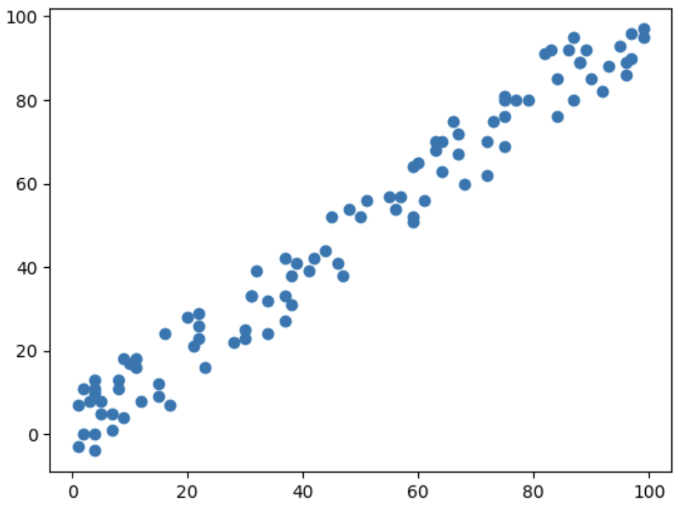
The relationship between two variables shows strong linearity and we may believe that the slope of line will be very close to $1$.

In order for expressing human’s belief into our probabilistic model, the bayesian statisticians usually introduce prior into the likelihood and update our belief by inferring posterior.

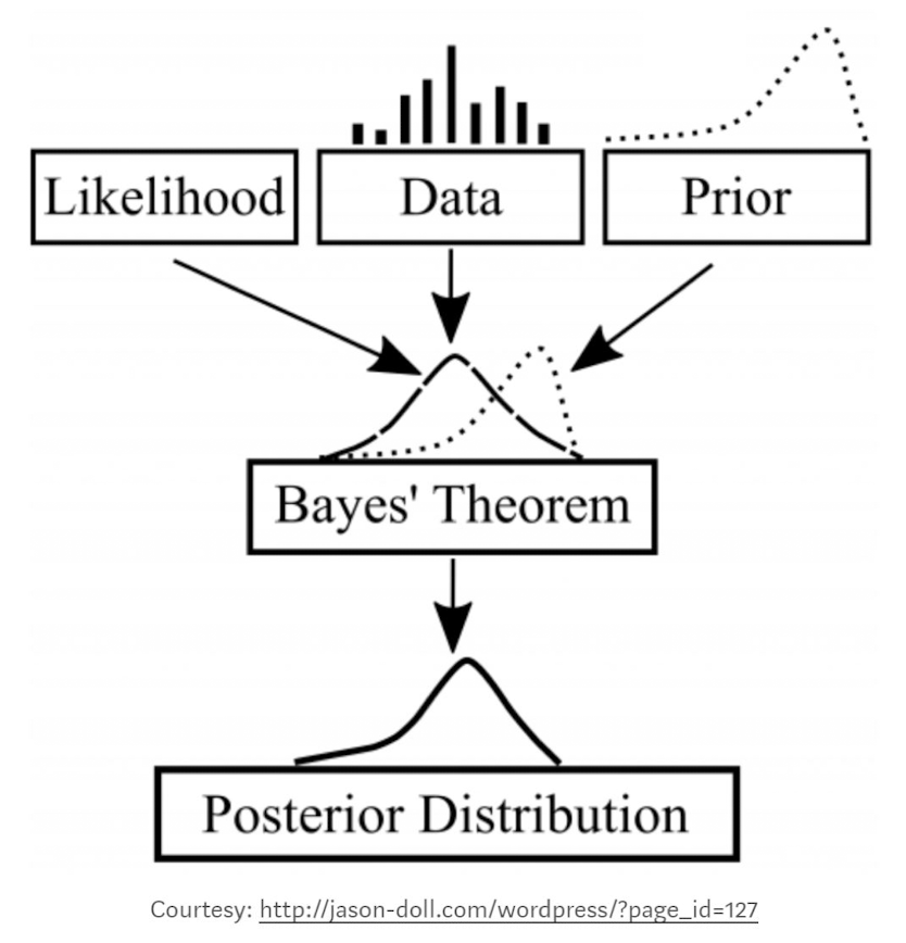
Similarly, maximum likelihood estimation can be naturally extended by Bayes Theorem. Instead of maximizing likelihood itself, we maximize posterior that incorporates our belief (prior). This augmented maximization is referred to as maximum a posterior (MAP) estimation:

\[\begin{aligned} X \sim p(\cdot \; | \; \theta) \Rightarrow \theta_{\text{MAP}} &= \underset{\theta}{\text{arg max }} \text{ log } p(\theta \; | \; X) \\ &= \underset{\theta}{\text{arg max }} \text{ log } p(X \; | \; \theta) \cdot p(\theta) \end{aligned}\]

Let’s apply this MAP for our Gaussian linear regression. For prior distribution, we usually choose the Gaussian for prior as Gaussian prior is conjugate prior of Gaussian likelihood. In other words, the posterior is in the same distribution class with prior, so the posterior will be Gaussian again.

\[\begin{aligned} p(\mathbf{w}) = \mathcal{N} ( \mathbf{w} \; | \; \mathbf{0}, \alpha \mathbf{I}) = \frac{1}{(2\pi)^{d/2}} \frac{1}{| \alpha \mathbf{I}|^{1/2}} \text{exp} \left( - \frac{1}{2 \alpha} \mathbf{w}^\top \mathbf{w} \right) \end{aligned}\]

Then, MAP of the whole dataset is

\[\begin{aligned} & \underset{\theta}{\text{ arg max }} \log p(\mathcal{D} \mid \theta) \cdot p(\theta) \\ = & \underset{\theta}{\text{ arg min}} \left[ \frac{1}{2 \sigma^2} \sum_{n=1}^N\left(y_n - \mathbf{w}^\top \mathbf{x}_n \right)^2 + \frac{1}{2 \alpha} \theta^\top \theta \right] \end{aligned}\]

Finally, we can see that maximizing posterior of Gaussian linear regression is equivalent to minimizing MSE loss with $L_2$ regularization. And it corresponds to our intuition: we regularize the optimal parameter by our prior belief of that.