[ML] Logistic Regression

Logistic Regression

Limitation of linear regression

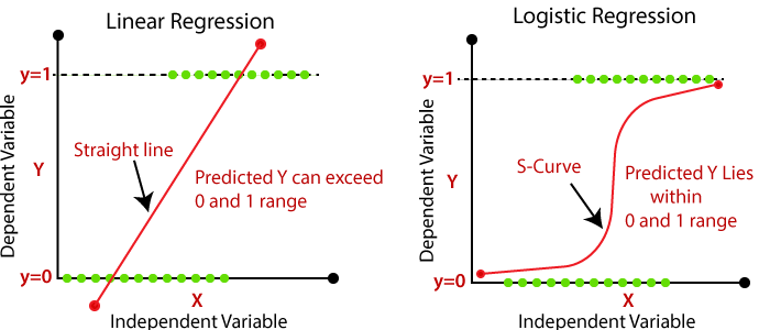
Then, can we use the linear regression model for binary classification? In this task, we represent the target values only by either $0$ or $1$ depending on the class. But in regression, the prediction range is usually continuous such as $(-\infty, \infty)$. How can we convert the real value prediction into discrete target value?

---

Logit Function

Odds and Probability

Let $N$ be the total number of trials, $n$ be the number of something happening, $p$ be the probability of happening something, and $o$ be the ratio of something happening to something not happening.

From $p = \frac{n}{N}$, we define odds $o = \frac{n}{N-n} = \frac{p}{1-p}$ as the fraction of success and failure. It may be more natural or more convenient than probabilities to represent likelihood of events.

Logit function

The definition of the logit function from $[0, 1]$ to $(-\infty, \infty)$ is

\[\begin{aligned} \text{logit }(p) := \text{log }(\frac{p}{1-p}) \end{aligned}\]

The inverse of the logit function, which is usually called logistic function, or in this case sigmoid function, is

\[\begin{aligned} \sigma (z) := \text{logit}^{-1}(p) = \frac{1}{1 + e^{-z}} \quad (-\infty < z < \infty) \end{aligned}\]

(But typically, sigmoid is considered as a special case of logistic function.)

As you can see, it is a squashing function that squashes the real value input $z$ to a range between $[0, 1]$. A key idea is that we can interpret this output as a probability between 0% ~ 100%. We can then set a rule, for example, if output is larger than 0.5, label as class 1, otherwise 0. In logistic regression, the logistic function maps the real value output of linear regression to the probability space. (So, it can be used for binary classification)

---

Logistic Regression

Let’s delve into how logistic regression works. Logistic regression is a statistical model that in its basic form uses a logistic function to model a binary dependent variable. The logit for the value labeled $1$ is equal to

\[\begin{aligned} z := \mathbf{w}^\top \mathbf{x} + \mathbf{b}. \end{aligned}\]

This implies that the odds are expressed by the exponential function

\[\begin{aligned} o = \frac{p}{1-p} = e^z = e^{\mathbf{w}^\top \mathbf{x} + \mathbf{b}} \to p = 1 - \frac{1}{1 + e^{\mathbf{w}^\top \mathbf{x} + \mathbf{b}}} \end{aligned}\]

It means the result of linear regression determines the probability of the label. So even though the probability may not be linear, the above arragement leads to a linear regression, as the decision boundary is still linear: $\mathbf{w}^\top \mathbf{x} + \mathbf{b} \geq \sigma^{-1}(0.5)$. The logistic regression gives the probability that an input vector belongs to a certain class. This means that the input space should be separated into two regions, one for each class, by a hyperplane $\mathbf{w}^\top \mathbf{x} + \mathbf{b} = 0$.

Cost Function: Binary Cross Entropy (BCE)

In binary classification task, we label one class by $y = 1$, and the other class by $y = 0$. And then we should maximize the probability of having the correct label, i.e., for datapoint $i$ whose class $y_i = 1$, should maximize $p^{(i)} = p(y_i = 1)$. Thus, it is natural to set the cost function to minimize as follows:

\[\begin{aligned} L(\mathbf{w}) = -\frac{1}{N} \sum_{i=1}^N \left[y_{i} \cdot \text{ log } p^{(i)} + (1 - y_{i}) \cdot \text{ log } (1 - p^{(i)}) \right] \end{aligned}\]

And, it is called binary cross entropy loss.

Maximum Likelihood Estimation

Mathematically, minimizing this loss is equivalent to the maximum likelihood estimate. To compute the likelihood, we need to compute $p(y_i = 1 | \mathbf{x}_i, \mathbf{w})$. First, consider the odds $e^\mathbf{z} = \frac{p}{1-p}$ and logit $\text{log }(\frac{p}{1-p}) = \mathbf{w}^\top \mathbf{x} + \mathbf{b}$.

Then, $p = \frac{1}{1 + e^{-\mathbf{w}^T \mathbf{x} - \mathbf{b}}} = \sigma (\mathbf{w}^\top \mathbf{x} + \mathbf{b})$

Consider the likelihood function of $(y_1, \cdots, y_N)$:

\[\begin{aligned} L(\mathbf{w}) = p(y_1, \cdots, y_N | \mathbf{x}_1, \cdots, \mathbf{x}_N, \mathbf{w}) = \prod_{i=1}^N p(y_i | \mathbf{x}_i, \mathbf{w}). \end{aligned}\]

Note that $p(y_i | \mathbf{x}_i, \mathbf{w}) = p(y_i = 1 | \mathbf{x}_i, \mathbf{w})^{y_i} \left(1 - p(y_i = 1 | \mathbf{x}_i, \mathbf{w}) \right)^{1-y_i}$. Thus,

\[\begin{aligned} L(\mathbf{w}) = \prod_{i=1}^N p(y_i = 1 | \mathbf{x}_i, \mathbf{w})^{y_i} \left(1 - p(y_i = 1 \| \mathbf{x}_i, \mathbf{w}) \right)^{1-y_i} \end{aligned}\]

Due to monotonicity of log function, it suffices to find $\mathbf{w}^* = \underset{\mathbf{w}}{\text{arg max}} \text{ log }L(\mathbf{w})$. Equivalently,

\[\begin{aligned} \mathbf{w}^* = \underset{\mathbf{w}}{\text{arg min}} \left[ - \sum_{i=1}^N y_i \cdot \text{ log } p(y_i = 1 | \mathbf{x}_i, \mathbf{w}) - \sum_{i=1}^N (1 - y_i) \cdot \text{ log } \left( 1 - p(y_i = 1 | \mathbf{x}_i, \mathbf{w}) \right) \right] \end{aligned}\]

By substituting $p(y_i = 1 | \mathbf{x}_i, \mathbf{w}) = \frac{1}{1 + e^{-\mathbf{w}^\top \mathbf{x}_i - \mathbf{b}}}$,

\[\begin{aligned} -\text{log } L(\mathbf{w}) &= \sum_{i=1}^N y_i \cdot \text{log}(1+e^{-\mathbf{w}^T \mathbf{x}_i}) + \sum_{i=1}^N (1-y_i) \cdot \mathbf{w}^\top \mathbf{x}_i + \sum_{i=1}^N (1-y_i) \cdot \text{log} (1+e^{-\mathbf{w}^\top \mathbf{x}_i}) \\ &= \sum_{i=1}^N \text{log} (1 + e^{-\mathbf{w}^\top \mathbf{x}_i}) + \sum_{i=1}^N (1-y_i) \cdot \mathbf{w}^\top \mathbf{x}_i. \end{aligned}\]

By differentiating $-\text{ log } L(\mathbf{w})$ with regard to $\mathbf{w}$, finally we get

\[\begin{aligned} \nabla_{\mathbf{w}} -\text{log } L(\mathbf{w}) &= -\sum_{i=1}^N \frac{e^{-\mathbf{w}^\top \mathbf{x}_i} \cdot \mathbf{x}_i}{1 + e^{-\mathbf{w}^\top \mathbf{x}_i - \mathbf{b}}} + \sum_{i=1}^N (1-y_i) \cdot \mathbf{x}_i \\ &= \sum_{i=1}^N \left[ \sigma(\mathbf{w}^\top \mathbf{x}_i + \mathbf{b}) - y_i \right] \cdot \mathbf{x_i}. \end{aligned}\]

---

Linear Multiclass Classification

But what if a number of classes is $C > 2$? Our simple logistic regression model can be extended by using a softmax instead of sigmoid. Before we look at softmax, how can represent the multiple classes? We need to convert the verbal label to numbers for mathematical model and functions. One of the most common way is the one-hot encoding. We should use the one-hot encoding to represent a category value because it is not ordinal (for input and output).

Linear Regression with Multiple Outputs

Now, assume that the total number of classes are $C > 2$. Can we simply extend the linear regression model to predict $C$ outputs? One solution can be applying linear regression to each output dimension (multiple linear regression). Note that the weight $\mathbf{w}$ is extended to a matrix, not a vector.

We may want the predictions for each class to be the probability like the one-hot vectors. Instead, to express the model more compactly, we can use linear algebra notation: vectors of probabilities. For example, $(\text{cat}, \text{chicken}, \text{dog}) = (0.2, 0.7, 0.1)$. But we cannot assure that the prediction is always stochastic; in other words positive, and the sum of them is $1$. This implies that we need to force them by normalizing the output of the linear model so that the sum becomes $1$ while all outputs are nonnegative. And it is exactly what softmax function does!

Softmax Function

In order to force the output of model to be stochastic, we can just apply additional one and onto function that outputs probabilites that are positive and sum to 1, just like sigmoid. Generally, the most used function in machine learning and deep learning is softmax :

\[\begin{aligned} \widehat{\mathbf{y}} = \text{softmax }(\mathbf{o}) \text{ where } \widehat{y}_i = \frac{e^{o_j}}{\sum_j e^{o_j}} \end{aligned}\]

The numerator and denominator make sure nonnegativity, and sum to $1$, respectively. To make a number positive, it can be any nonnegative functions like $x^2$, $| x |$, and $\text{ReLU}$. But softmax employs an exponential function as it is especially convenient because it’s not only one to one and onto that maps $\mathbb{R}$ to entire set of positives, but also easily differentiable.

• Why it is called “softmax” [3]
  

The original form of softmax has the temperature hyperparameter $\tau$:

\[\begin{aligned} \widehat{y}_i = \frac{e^{o_j / \tau}}{\sum_j e^{o_j / \tau}} \end{aligned}\]

When $\tau$ is low, it becomes a distribution sampling the max value most of the time (depending on $\tau$). So, by tweaking $\tau$, the maximum probability can be adjusted to be hard or soft.

The importance of softmax is due to differentiability; being differentiable is important in many applications. Unlike $\text{max}()$, which is not differentiable, $\text{softmax}()$ is differentiable clearly regardless of value of $\tau$.

Loss Function for Classification

We need to extend not only sigmoid, but also the loss function. Cross-Entropy loss , which is usually referred to as negative-log-likelihood (nll) loss , is a general version of binary cross entropy, which is equivalent to maximum-likelihood for classification

\[\begin{aligned} L(\mathbf{w}) = \prod_{i=1}^{n} P(y^{(i)} | \mathbf{x}^{(i)}) \to -\text{log } L(\mathbf{w}) = \sum_{i=1}^{n} -\text{log } P(y^{(i)} | \mathbf{x}^{(i)}) \end{aligned}\]

where

\[\begin{aligned} P(y|x) = \prod_{j=1}^{C} \widehat{y}_{j}^{y_j} \end{aligned}\]

( $y_j$ is the actual probability of class $j$, and $\widehat{y}_j$ is the predicted probability of class $j$.)

Thus, $l(\mathbf{w}) = - \sum_{i=1}^{n} \sum_{k = 1}^{C} y_{j}^{(i)} \cdot \text{ log } p(y^{(i)} = k | \mathbf{x}^{(i)})$. The reason why this loss equation is referred to as cross entropy loss is, it can be interpreted as the cross entropy $-\mathbb{E}_p [\text{log } q(X)]$ where $p$ is the true distribution of target and $q$ is the estimated, predicted distribution of $p$.

• Gradient

The softmax function is a non-linear function (due to exponential function). Thus, we don’t have a closed form solution. This means that we need to use the gradient descent method. The gradient of CE loss can be obtained as the error times the input value:

\(\begin{aligned} \nabla_{w_k} L(\mathbf{w}) = \frac{1}{N} \sum_{i=1}^N (\widehat{y}_{k}^{(i)} - y_{k}^{(i)}) \mathbf{x}^{(i)} \end{aligned}\)

For derivation,

\[\begin{aligned} l(\mathbf{w}) &= - \frac{1}{N} \sum_{i=1}^{N} \sum_{k = 1}^{C} y_{j}^{(i)} \cdot \text{ log } p(y^{(i)} = k | \mathbf{x}^{(i)}) \\ &= - \frac{1}{N} \sum_{i=1}^{N} \sum_{k = 1}^{C} y_{k}^{(i)} \cdot \text{ log } \frac{e^{\mathbf{w}_k^\top \mathbf{x}^{(i)}}}{\sum_{j=1}^C e^{\mathbf{w}_j^\top \mathbf{x}^{(i)}}} \\ &= - \frac{1}{N}\sum_{i=1}^{N} \sum_{k = 1}^{C} y_{j} \cdot (\mathbf{w}_k^\top \mathbf{x}^{(i)} - \text{ log } (\sum_{j=1}^C e^{\mathbf{w}_j^\top \mathbf{x}^{(i)}})), \\ \\ N \cdot \frac{\partial l(\mathbf{w})}{\partial w_{mn}} &= - \sum_{i=1}^{N} y_{m}^{(i)} \cdot x_{n}^{(i)} + \sum_{i=1}^{N} \sum_{k = 1}^{C} y_{k}^{(i)} \cdot \frac{ e^{\mathbf{w_k}^\top \mathbf{x_i}} }{ \sum_{j=1}^C e^{\mathbf{w_j}^\top \mathbf{x}^{(i)}}} \cdot x_{k}^{(i)}, \\ \\ \frac{\partial l(\mathbf{w})}{\partial w_{mn}} &= - \frac{1}{N} \sum_{i=1}^{N} \left[ y_m^{(i)} - p_m (\mathbf{x}^{(i)}) \right] \cdot x_{n}^{(i)}._\blacksquare \end{aligned}\]

Decision Boundaries

The following figure shows the area of 3 flower types with respect to 2 features: the width and length of petal.

Again, even if the softmax is non-linear, we can observe that the boundaries between each two classes become linear. Always remember that sigmoid and softmax are just served as squashing function!

---

Reference

[1] Christopher M. Bishop, Pattern Recognition and Machine Learning, Springer 2006.
[2] GeÌron, Aureìlien, Hands-on Machine Learning with Scikit-Learn, Keras and TensorFlow: Concepts, Tools, and Techniques to Build Intelligent Systems. 2nd ed., O’Reilly 2019.
[3] Why is softmax activate function called “softmax”?