
[Measure Theory] Differentiation
The inverse relationship between differentiation and integration was already grasped in the early stages of basic calculus. And the Radon-Nikodym theorem indeed provides an abstract notion of the “derivative” of a signed measure $\nu$ with respect to a measure $\mu$. In this post, we analyze more deeply the special case when $(X, \mathcal{A}) = (\mathbb{R}^n, \mathcal{B}_{\mathbb{R}^n})$ and $\mu = m$ is Lebesgue measure and want to look at when the function is differentiable and when the fundamental theorem of calculus holds.
In brief summary, we will show that
- The derivative of $\int_a^x f(y) \; dy$ exists and is equal to $f$ a.e. if $f$ is integrable.
- $\int_a^b f^\prime (y) \; dy = f(b) - f(a)$ if $f$ is absolutely continuous.
And this result is known as the fundamental theorem of Calculus for Lebesgue integration.
Maximal Functions
Motivation
Suppose an integrable function $f: [a, b] \to \mathbb{R}$ is given, and let
\[\begin{aligned} F(x) = \int_a^x f(y) \; dy \quad (a \leq x \leq b). \end{aligned}\]Recall the definition of the derivative, and $F^\prime (x)$ is given as the limit of the following quotient:
\[\begin{aligned} \frac{1}{h} \int_{x}^{x + h} f(y) \; dy = \frac{1}{| I |} \int_I f(y) \; dy, \end{aligned}\]where $I = (x, x+h)$ and $| I |$ is the length of the interval. Here, to give the motivation let’s just assume that $h > 0$. By naturally extending our discussion on $\mathbb{R}^n$, then our question is now reformulated as
\[\begin{aligned} \lim_{r \to 0} \frac{1}{m(B(x, r))} \int_{B(x, r)} f(y) \; dy = f(x) \text{ for a.e } x \text{?} \end{aligned}\](Of course, note that in the special case when $f$ is continuous at $x$, the limit does converge to $f(x)$.) To deal with this kind of averaging problem, we will construct some quantitative estimates relevant to the overall behavior of the averages of $f$. And this will be achieved by considering the maximal averages of $| f |$ so called maximal function defined by
\[\begin{aligned} \underset{r > 0}{\text{ sup }} \frac{1}{m(B(x, r))} \int_{B(x, r)} | f(y) | \; dy, \end{aligned}\]to which we now turn. The maximal function we examine here originally emerged in Hardy and Littlewood’s treatment of the one-dimensional scenario: how the player’s score in cricket could be distributed to maximize their satisfaction. Remarkably, these concepts hold universal significance in the realm of analysis.
Vitali covering lemma
For further discussion, the following lemma is quite useful, which is known as Vitali covering lemma:
Suppose $E \subset \mathbb{R}^n$ is covered by a collection of open balls $\{ B_{\alpha} \}$ and they are uniform bounded. (In other words, there exists a positive real number $R$ such that the diameter of each $B_{\alpha}$ is bounded by $R$.)
Then, there exists a disjoint sequence $B_1, B_2, \cdots$ of elements of $\{ B_{\alpha} \}$ such that $$ \begin{aligned} m (E) \leq 5^n \sum_{k} m (B_k). \end{aligned} $$
$\mathbf{Proof.}$
The idea of proof is quite intuitive.
- Choose one open ball on the large side, i.e. with the radius larger than the half of the supremum of radiuses.
- Choose another open ball on the large side, but is disjoint with the chosen ball in the previous step.
- Repeat the steps inductively.
Let $d(B_{\alpha})$ be the diameter of $B_{\alpha}$. Note that $\underset{\alpha}{\text{ sup }} d(B_{\alpha})$ is bounded by $R$. Choose $B_1$ such that
\[\begin{aligned} d (B_1) \geq \frac{1}{2} \underset{\alpha}{\text{ sup }} d(B_{\alpha}). \end{aligned}\]Inductively, for $k \geq 1$, once $B_1, \cdots B_k$ are chosen, choose $B_{k+1}$ disjoint from $B_1, \cdots, B_k$ such that
\[\begin{aligned} d (B_{k + 1}) \geq \frac{1}{2} \underset{\alpha}{\text{ sup}} \left\{ d(B_{\alpha}) \mid B_{\alpha} \text{ is disjoint from } B_1, \cdots, B_k \right\}. \end{aligned}\]The procedure might terminate after a finite number of steps or it might not.
If $\sum_{k} m (B_k) = \infty$, then we prove the result. Suppose $\sum_{k} m (B_k) < \infty$ so that $d(B_k) \to 0$ as $k \to \infty$. And let $B_k^*$ be the ball with the same center as $B_k$ but 5 times the radius.
We will show that every element $B_\alpha$ in open cover can be covered by one of $B_k^*$, which implies the result.
$\mathbf{Proof.}$
Fix $\alpha$. From $d(B_k) \to 0$ as $k \to \infty$, let $k$ be the smallest integer such that
\[\begin{aligned} d (B_{k+1}) < \frac{1}{2} d(B_\alpha) \end{aligned}\]or \(\{ B_j \}\) is terminated at $B_k$.
$B_\alpha$ must intersect one of $B_1, \dots B_k$ by our construction, or else we would have chosen it instead of $B_{k+1}$. Hence, we can find the smallest positive integer $j_0 \leq k$ such that $B_\alpha \cap B_{j_0} \neq \emptyset$. Then we have
\[\begin{aligned} d(B_{j_0}) \geq \frac{1}{2} d(B_\alpha) \end{aligned}\]as $B_\alpha$ is disjoint with $B_1, \dots B_{j_0 - 1}$ by definition of $j_0$ and we selected $B_{j_0}$ that has the radius larger than the half of open balls disjoint with $B_1, \dots B_{j_0 - 1}$, which contains $B_{\alpha}$.
Note that
\[\begin{aligned} B_{\alpha} \subset B_{j_0}^*. \end{aligned}\]
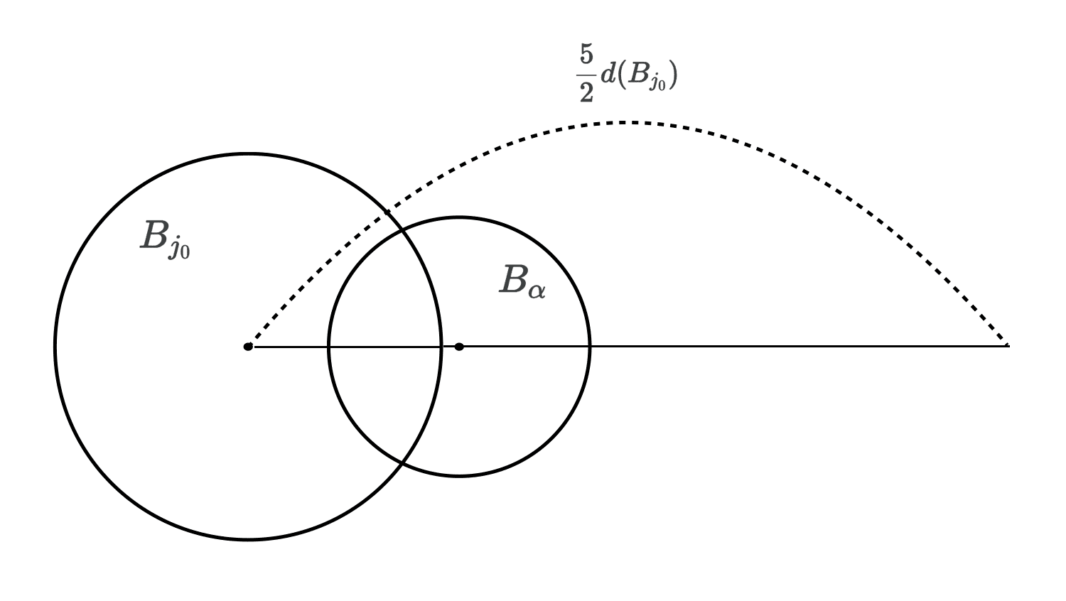
This can be shown in the mathematical statement, too. Choose $y \in B_{\alpha} \cap B_{j_0}$. Let $x_{j_0}$ be the center of $B_{j_0}$. For any $x \in B_{\alpha}$, we have
\[\begin{aligned} | x - x_{j_0} | & \leq | x - y | + | y - x_{j_0} | \\ & < d (B_\alpha) + \frac{1}{2} d(B_{j_0}) \\ & \leq 2 d(B_{j_0}) + \frac{1}{2} d(B_{j_0}) = \frac{5}{2} d(B_{j_0}). \end{aligned}\]And this shows that any open balls $B_{\alpha}$ in the collection of open balls \(\{ B_{\alpha} \}\) that cover $E$ is contained in at least one of the enlarged open ball. Done.
\[\tag*{$\blacksquare$}\]The lemma states that for any covers consist of infinite number of uniform bounded open balls of the area $E$, disjoint subcollection can be selected and by enlarging each with five times the radius, it is possible to cover $E$.
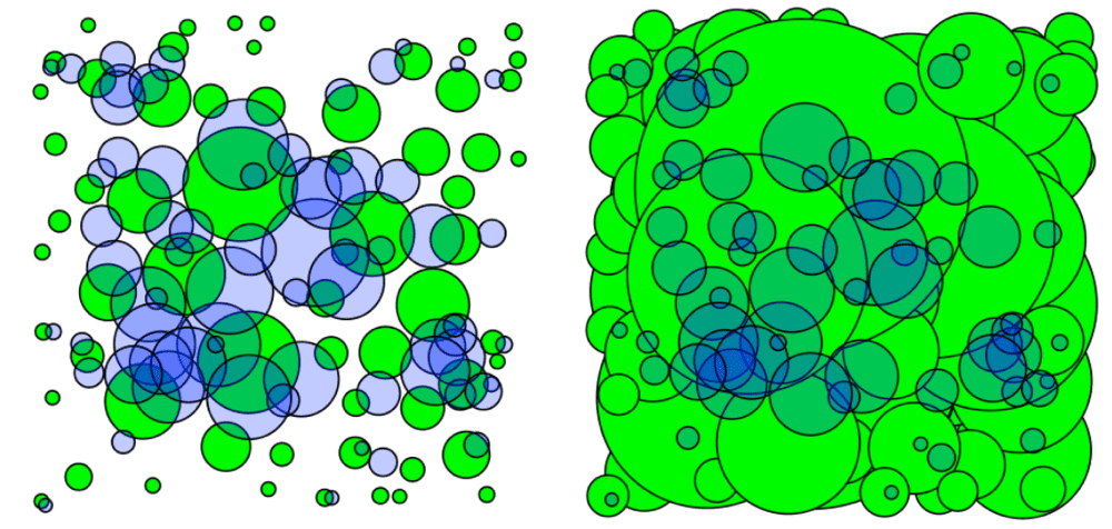
$\mathbf{Fig\ 1.}$ Left: open ball covers Right: the subcollection with three times the radius
(source: [3])
But one should note that the uniform boundedness is necessary; consider \(E = \mathbb{R}^2 \times \{ 0 \}\subset \mathbb{R}^3\), and the following cover on $xy$-plane:
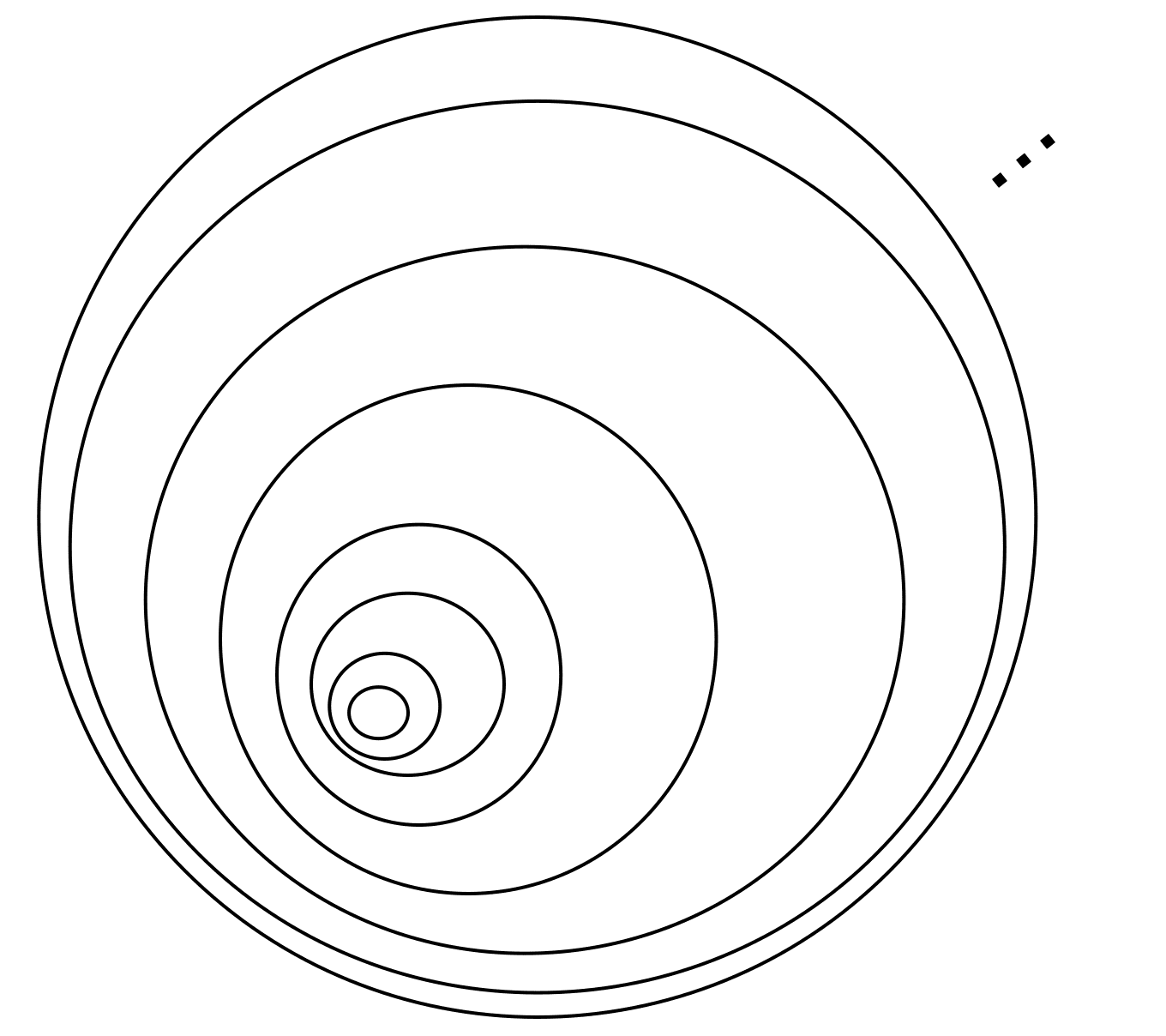
$\mathbf{Fig\ 2.}$ Counterexample when uniform boundedness is not ensured
Maximal Theorem
Now we define the maximal function. In our exploration of the Lebesgue integral thus far, we have worked under the assumption that $f$ is integrable. This “global” assumption stands slightly apart from the context of a “local” notion such as differentiability. Indeed, Lebesgue differentiation theorem involves a limit taken over balls that shrink to the point $x$, therefore the behavior of $f$ far from $x$ is irrelevant. Thus, we anticipate the result to remain valid even if we simply loosen integrability of $f$ on the entire domain to every ball. Formally, we define the new notion of integrability called locally integrability:
$f$ is locally integrable if $$ \begin{aligned} \int_K | f(x) | \; dx < \infty \quad \text{ whenever } \quad K \text{ is compact.} \end{aligned} $$ And, if $f$ is locally integrable, define $$ \begin{aligned} Mf(x) = \underset{r > 0}{\text{ sup }} \frac{1}{m(B(x, r))} \int_{B(x, r)} | f(y) | \; dy. \end{aligned} $$ The function $Mf$ is called the maximal function of $f$. (Note that without supremum, we are looking at the average of $| f |$ over $B(x, r)$.)
Here are some example plots of $Mf$ for given $f$:
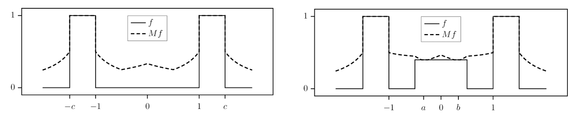
$\mathbf{Fig\ 3.}$ Plots for $f$ and $Mf$ (source: [4])
It is possible to show that $Mf$ is a Lebesuge measurable function. If $f$ is locally integrable, for each $r > 0$ the function $h (x) = \int_{B(x, r)} | f(y) | \; dy$ is continuous by
\[\begin{aligned} \int_{B(x, r)} | f(y) | \; dy - \int_{B(\tilde{x}, r)} | f(y) | \; dy & = \int | f(y) | ( \chi_{B(x, r)} - \chi_{B(\tilde{x}, r)}) (y) \; dy \\ & \to 0 \end{aligned}\]as $\tilde{x} \to x$ by dominated convergence theorem. Note that for a metric space, sequential continuity implies continuity for a function. Then
\[\begin{aligned} \{ x \mid Mf (x) > a \} & = \bigcup_{r > 0} \left\{ x \; \middle| \; \int_{B(x, r)} | f(y) | \; dy > a \cdot m (B(x, r)) = a r^n \right\} \end{aligned}\]is open due to continuity. But $Mf$ is not integrable, even though $f$ is integrable. Consider $f = \chi_B$ where $B = B(0, 1)$ unit ball. Then $Mf(x)$ is approximately a constant times $1 / | x |^n$ for $| x | \gg 1$, therefore, not integrable.
We consider now an inequality called weak 1-1 inequality. It is also known as maximal theorem, or Hardy–Littlewood maximal inequality (Weak type). It is so named because $M$ does not map integrable functions into integrable functions as we saw, but approximates this behavior in a certain sense. For a measure space $(X, \mathcal{A}, \mu)$, define $\lambda_g: \mathbb{R}_{>0} \to \mathbb{R}$ as
\[\begin{aligned} \lambda_g (\beta) := \mu \left( \{ x \in X : | g(x) | > \beta \} \right) \end{aligned}\]In the jargon of $L^p$ space, we say $f$ is weak $L^1$ if $\beta \lambda_f (\beta)$ is bounded. And the following theorem states that $M$ maps an integrable function $f$ to weak-$L^1$ $Mf$:
If $f$ is integrable, for all $\beta > 0$, $$ \begin{aligned} m ( \{ x : Mf(x) > \beta\} ) \leq \frac{5^n}{\beta} \int | f(x) | \; dx \end{aligned} $$
$\mathbf{Proof.}$
Let any $\beta > 0$ be given. Define
\[\begin{aligned} E_{\beta} = \{ x \mid Mf(x) > \beta \}. \end{aligned}\]Now, we will find the collection of open balls that covers $E_{\beta}$. If $x \in E_{\beta}$, then $Mf(x) > \beta$, thus there exists $r > 0$ such that $\frac{1}{m(B(x, r))} \int_{B(x, r)} | f(y) | \; dy > \beta$. Hence,
\[\begin{aligned} d(B(x, r)) = m (B (x, r)) < \frac{1}{\beta} \int_{B(x, r)} | f(y) | \; dy \leq \frac{1}{\beta} \int | f (y) | \; dy. \end{aligned}\]Denote this ball $B(x, r)$ by $B_x$. Then, $E_{\beta}$ is covered by \(\{ B_x \}_{x \in E_\beta}\), where the diameter of $B_x$ is uniform bounded. By Vitali covering lemma, we can extract a disjoint sequence $B_1, B_2, \cdots$ such that
\[\begin{aligned} m (E_\beta) \leq 5^n \sum_{k} m (B_k) \end{aligned}\]Hence
\[\begin{aligned} m(E_\beta) & \leq 5^n \sum_{k} m (B_k) \\ & \leq \frac{5^n}{\beta} \sum_{k} \int_{B_k} | f(y) | \; dy \\ & = \frac{5^n}{\beta} \int_{\bigcup_{k} B_k} | f(y) | \; dy \\ & \leq \frac{5^n}{\beta} \int | f(y) | \; dy. \end{aligned}\] \[\tag*{$\blacksquare$}\]Lebesgue Differentiation Theorem
The key to using maximal functions to study differentiation is the following theorem. With maximal theorem in hand, we now present the Lebesgue differentiation theorem. It posits that the estimate obtained for the maximal function now leads to the desired solution of our antiderivative problem. For more general versions for theorem, see [5].
In the proofs, we use the notion of limit superior for real-valued functions
\[\begin{aligned} \limsup _{r \rightarrow R} \phi(r)=\lim _{\epsilon \rightarrow 0} \sup _{0<|r-R|<\epsilon} \phi(r)=\inf _{\epsilon>0} \sup _{0<|r-R|<\epsilon} \phi(r). \end{aligned}\]One can easily verify that
\[\begin{aligned} \lim _{r \rightarrow R} \phi(r)=c \quad \text { iff } \quad \limsup _{r \rightarrow R}|\phi(r)-c|=0 \end{aligned}\]$\mathbf{Proof.}$
Step 1: Assume that $f$ is continuous
Fix any $x \in X$. There exists $\delta > 0$ for any $\varepsilon > 0$ such that $| f(y) - f(x) | < \varepsilon$ whenever $| y - x | < \delta$. Then from
\[\begin{aligned} f_r (x) - f(x) = \frac{1}{m(B(x, r))} \int_{B(x, r)} ( f(y) - f(x) ) \; dy, \end{aligned}\]we have
\[\begin{aligned} | f_r (x) - f(x) | \leq \frac{1}{m(B(x, r))} \int_{B(x, r)} | f(y) - f(x) | \; dy \to 0 \end{aligned}\]as $r \to 0$ by the continuity of $f$.
Step 2: Assume now that $f$ is locally integrable.
It suffices to show that for each $N$, $f_r (x) \to f(x)$ for almost every $x \in B(0, N)$ as $r \to 0$. Fix $N$. Then without loss of generality we may assume $f$ is $0$ outside of $B(0, 2N)$ and integrable. It is because if we define
\[\begin{aligned} \tilde{f}(x) = \begin{cases} f(x) & \quad | x | \leq 2N \\ 0 & \quad | x | > 2N. \end{cases} \end{aligned}\]$\tilde{f} = 0$ for $x \notin \overline{B(0, 2N)}$ and $\tilde{f} = f$ for $x \in \overline{B(0, 2N)}$ so that $\tilde{f}$ is integrable.
Recall that a Lebesgue measurable real-valued integrable function $f$ is possible to be approximated by continuous function $g$ with compact support in the sense of $L^1$ norm (see my previous posts):
\[\begin{aligned} \int | f - g | < \varepsilon. \end{aligned}\]Therefore, for each $r > 0$,
\[\begin{aligned} | f_r (x) - f(x) | \leq | f_r (x) - g_r (x) | + | g_r (x) - g(x) | + | g(x) - f(x) | \end{aligned}\]Note that the second term in RHS goes to $0$ as $r \to 0$ for a fixed $x$ by continuity. Fix $\beta > 0$. From $a + b > \beta \rightarrow \alpha > \beta / 2$ or $b > \beta / 2$, we have
\[\begin{aligned} m( \{ x : \limsup _{r \to 0} | f_r (x) - f(x) | > \beta \}) \leq \; & m \left(\left\{ x : \limsup _{r \to 0} | f_r (x) - g_r(x) | > \frac{\beta}{2} \right\}\right) \\ & + m \left(\left\{ x : | g (x) - f(x) | > \frac{\beta}{2} \right\}\right) \\ \leq \; & m \left( \left\{ x : M(f - g) (x) > \frac{\beta}{2} \right\} \right) \\ & + m \left(\left\{ x : | f - g | (x) > \frac{\beta}{2} \right\}\right) \\ \leq \; & \frac{2 \cdot 5^n}{\beta} \int | f - g | + \frac{2}{\beta} \int | f - g | < \frac{2 \cdot (5^n + 1)}{\beta} \varepsilon \end{aligned}\]where the last step is derived by maximal theorem and Chebyshev’s inequality. Since $\varepsilon > 0$ is arbitrary,
\[\begin{aligned} m( \{ x : \limsup _{r \to 0} | f_r (x) - f(x) | > \beta \}) = 0. \end{aligned}\]for any $\beta > 0$. Thus,
\[\begin{aligned} m ( \{ x : \limsup _{r \to 0} | f_r (x) - f (x) | > 0 \}) \leq \sum_{j=1}^\infty m\left(\left\{ x : \limsup _{r \to 0} | f_r (x) - f(x) | > \frac{1}{j} \right\}\right) = 0, \end{aligned}\]which proves the theorem.
\[\tag*{$\blacksquare$}\]In fact, we can get a slightly stronger statement of the last theorem easily:
$\mathbf{Proof.}$
Note that for each $c \in \mathbb{R}$, $\tilde{f}(y) = | f(y) - c |$ is locally integrable, too. By the last theorem we can choose a measurable set $N_c$ of measure zero such that for $x \notin N_c$,
\[\begin{aligned} \frac{1}{m(B(x, r))} \int_{B(x,r)} | f(y) - c | \; dy \to | f(x) - c | \end{aligned}\]as $r \to 0$. Then let $N = \bigcup_{c \in \mathbb{Q}} N_c$. It is clear that $m (N) = 0$. We claim that for any $\varepsilon > 0$,
\[\begin{aligned} \limsup _{r \to 0} \frac{1}{m(B(x, r))} \int_{B(x, r)} | f(y) - f(x) | \; dy < 2 \varepsilon \end{aligned}\]for all $x \notin N$, which implies the result.
To prove the claim, fix $x \notin N$ and we can choose $\tilde{c} \in \mathbb{Q}$ such that $| f(x) - \tilde{c} | < \varepsilon$ as $\mathbb{Q}$ is dense in $\mathbb{R}$. Then
\[\begin{aligned} \frac{1}{m(B(x, r))} \int_{B(x, r)} | f(y) - f(x) | \; dy \leq \; & \frac{1}{m(B(x, r))} \int_{B(x, r)} | f(y) - \tilde{c} | \; dy \\ & + \frac{1}{m(B(x, r))} \int_{B(x, r)} | f(x) - \tilde{c} | \; dy \\ = \; & \frac{1}{m(B(x, r))} \int_{B(x, r)} | f(y) - \tilde{c} | \; dy + | f(x) - \tilde{c} | \end{aligned}\]Hence
\[\begin{aligned} \limsup _{r \rightarrow 0} \frac{1}{m(B(x, r))} \int_{B(x, r)}|f(y)-f(x)| \; d y \leq 2|f(x)- \tilde{c}| < 2 \varepsilon \end{aligned}\] \[\tag*{$\blacksquare$}\]As an application of the theorem, we introduce the new notion:
Antiderivatives
Now let’s consider real-valued functions on the real line $\mathbb{R}$. By the results on maximal functions, we can show that the derivative of the antiderivative of an integrable function is the function itself.
Define the indefinite integral or antiderivative $F$ of an integrable function $f$ by
\[\begin{aligned} F (x) = \int_a^x f(t) \; dt. \end{aligned}\]It is trivial that $F$ is continuous. Then, the following is satisfied:
- $F$ is differentiable almost everywhere;
- $F^\prime (x) = f(x)$ a.e.
$\mathbf{Proof.}$
If $h > 0$, we have
\[\begin{aligned} F(x + h) - F(x) = \int_x^{x + h} f(y) \; dy, \end{aligned}\]therefore
\[\begin{aligned} \left| \frac{F(x+h) - F(x)}{h} - f(x) \right| & = \frac{1}{h} \left| \int_{x}^{x+h} (f(y) - f(x)) \; dy \right| \\ & \leq 2 \frac{1}{m (B(x, h))} \int_{x-h}^{x+h} | f(y) - f(x) | \; dy. \end{aligned}\]By the previous theorem, the RHS converges to $0$ as $h \to 0$ for almost everywhere. The left hand derivative (when $h < 0$) can be handled similarly.
\[\tag*{$\blacksquare$}\]In the later section, we will show that the antiderivative is continuous, and indeed absolutely continuous.
Increasing Functions
Our next goal is to show that functions of bounded variation differentiable almost everywhere. But as a priori, in this section we show that increasing functions are differentiable almost everywhere. We start with right continuous increasing functions.
By the Lebesgue decomposition theorem a finite measure on the real line can be decomposed into a part that is absolutely continuous with respect to Lebesgue measure and a part that is mutually singular with respect to Lebesgue measure. We first deal with the mutually singular part. And, we will see that the Radon-Nikodym derivative from the absolutely continuous part will be the derivative for the function!
$\mathbf{Proof.}$
Since $\lambda \perp m$, there exist measurable sets $E$ and $F$ such that $\lambda (F) = m (E) = 0$ and $F = E^c$. For $\beta > 0$, let
\[\begin{aligned} A_{\beta} = \left\{ x \in F \cap [0, 1] : \limsup _{r \to 0} \frac{\lambda (B(x, r))}{m (B(x, r))} > \beta \right\} \end{aligned}\]Then
\[\begin{aligned} \left\{ x \in F \cap [0, 1] : \limsup _{r \to 0} \frac{\lambda (B(x, r))}{m (B(x, r))} > \beta \right\} = \bigcup_{k=1}^\infty A_{\frac{1}{k}} \end{aligned}\]Hence, it suffices to show $m (A_\beta) = 0$ for all $\beta > 0$.
Let $\varepsilon > 0$. As $\lambda$ is a Lebesgue-Stieltjes measure, we can choose an open set $G^\prime$ containing $F$ such that $\lambda (G^\prime - F) < \varepsilon$. Since $\lambda (F) = 0$, we have $\lambda (G^\prime) < \varepsilon$.
Set $G = G^\prime \cap [-1, 2]$. Then $G$ is a bounded open set satisfying $F \cap [0, 1] \subset G^\prime \cap [0, 1] \subset G$ and $\lambda (G) < \varepsilon$.
If $x \in A_{\beta}$, then $x \in F \cap [0, 1] \subset G$. Thus we can choose an open ball $B_x$ centered at $x$ such that
\[\begin{aligned} B_x \subset G \text{ and } \lambda (B_x) > \beta m (B_x) \end{aligned}\]By Vitali covering lemma, we can find a disjoint subsequence $B_1, B_2, \cdots$ such that
\[\begin{aligned} m(A_\beta) & \leq 5 \sum_{n=1}^\infty m (B_n) \\ & \leq \frac{5}{\beta} \sum_{n=1}^\infty \lambda (B_n) \\ & \leq \frac{5}{\beta} \lambda (G) = \frac{5}{\beta} \varepsilon. \end{aligned}\]Since $\varepsilon$ is arbitrary, $m(A_\beta) = 0$.
\[\tag*{$\blacksquare$}\]Here is our result on differentiation for right continuous increasing functions.
$\mathbf{Proof.}$
It is enough to show that $F$ is differentiable on $[0, 1]$. Once we have that, the same argument can be used to show that $F$ is differentiable a.e. on $[-N, N]$ for each $N \in \mathbb{N}$, and that proves that $F$ is differentiable a.e. on $\mathbb{R}$. If we redefine $F$ so that
\[\begin{aligned} F(x) = \begin{cases} \lim _{y \to 0^+} F(y) & \quad x \leq 0 \\ F(x) & \quad x \in (0, 1] \\ F(1) & \quad x \geq 1 \end{cases} \end{aligned}\]then $F$ is still right continuous and increasing, and we have not affected the differentiability of $F$ on $[0, 1]$ except possibly at the points $0$ and $1$.
Let $\nu$ be the Lebesuge-Stieltjes measure defined by $F$. By the Lebesgue decomposition theorem, $\nu = \lambda + \rho$ where $\lambda \perp m$, $\rho \ll m$, and $\lambda$ and $\rho$ are positive measures. By the Radon-Nikodym theorem, there exists a non-negative integrable function $f$ such that $\rho (A) = \int_A f \; dm$ for each measurable $A$.
Let
\[\begin{aligned} H (x) = \lambda((0, x]) = F(x) - F(0) - \int_0^x f(y) \; dy. \end{aligned}\]Since $f$ is integrable, we know that $\int_0^x f(y) \; dy$ is differentiable. Note that $\int_0^x f(y) \; dy$ is continuous with respect to $x$ due to the dominated convergence theorem and increasing because $f$ is non-negative. Hence, $H$ is right-continuous, increasing, and $H(0) = 0$.
Thus $\lambda$ is the Lebesgue-Stieltjes measure define in terms of $H$. By the previous lemma,
\[\begin{aligned} \limsup _{h \to 0+} \frac{H (x+h) - H(x)}{h} & \leq \limsup _{h \to 0+} \frac{H (x + h) - H(x - h)}{h} \\ & = \limsup _{h \to 0+} \frac{\lambda ((x - h, x+h])}{h} \\ & \leq 4 \limsup _{h \to 0+} \frac{\lambda (B(x, 2h))}{4h} = 0 \end{aligned}\]for almost every $x$. The same is true for the left hand derivative. Hence $H$ is differentiable a.e. $x$ with $H^\prime = 0$ a.e. Thus, $F$ is differentiable a.e. $x$ with $F^\prime (x) = f(x)$.
If $a < b$, then
\[\begin{aligned} \int_a^b F^\prime (x) \; dx & = \int_a^b f(x) \; dx \\ & = \rho ((a, b]) \\ & \leq \nu ((a, b]) \\ & = F(b) - F(a). \end{aligned}\] \[\tag*{$\blacksquare$}\]Finally, we obtain the main theorem on the differentiation of increasing functions. The previous proposition with respect to right continuous increasing function can be extended to general increasing functions:
$\mathbf{Proof.}$
Since $F$ is increasing, $F$ is continuous except at most countably many values of $x$. (It is because for each $x$ where $f (x-) < f (x+)$ there is a rational number in the interval $(f (x-), f (x+))$. No two such intervals can intersect because $f$ is increasing, so the rational numbers corresponding to different intervals must be different, and we conclude that there can only be countably many $x$ such that $f (x-) \neq f (x+)$.)
Define $G(x) = \lim _{y \to x +} F(y)$, which is increasing and right continuous. Then $G(x) = F(x)$ a.e. And it is differentiable a.e. by the previous proposition. Let $x$ be a point where $G$ is differentiable and $F(x) = G(x)$. We claim the following:
$\mathbf{Proof.}$
Set $\varepsilon > 0$. Let $h > 0$. Then there exists $x_h \in (x + h, x + (1 + \varepsilon) h)$ such that $F(x_h) = G(x_h)$. Then
\[\begin{aligned} F(x+h) \leq F(x_h) = G(x_h) \leq G(x + (1 + \varepsilon) h). \end{aligned}\]Thus
\[\begin{aligned} \frac{F(x+h) - F(x)}{h} \leq \frac{G(x + (1+\varepsilon)h) - G(x)}{h} = \frac{G(x + (1+\varepsilon)h) - G(x)}{h (1 + \varepsilon)} (1 + \varepsilon) \end{aligned}\]Similarly, there exists $x_h \in (x + (1 - \varepsilon) h, x + h)$ such that $F(x_h) = G(x_h)$. Then
\[\begin{aligned} \frac{F(x+h) - F(x)}{h} \geq \frac{F(x_h) - G(x)}{h} & \geq \frac{G(x_h) - G(x)}{h} \\ & \geq \frac{G(x + (1-\varepsilon)h) - G(x)}{h (1 - \varepsilon)} (1 - \varepsilon). \end{aligned}\]Therefore
\[\begin{aligned} \limsup _{h \to 0+} \frac{F(x+h) - F(x)}{h} & \leq (1 + \varepsilon) G^\prime (x) = (1 + \varepsilon) L \\ \limsup _{h \to 0+} \frac{F(x+h) - F(x)}{h} & \geq (1 - \varepsilon) G^\prime (x) = (1 - \varepsilon) L \end{aligned}\]Since $\varepsilon$ is arbitrary, $\lim _{h \to 0+} \frac{F(x+h) - F(x)}{h} = L$. Similarly, one can show that $\lim _{h \to 0-} \frac{F(x+h) - F(x)}{h} = L$.
\[\tag*{$\blacksquare$}\]Note that $G^\prime$ is locally integrable by the previous proposition. Since $F^\prime = G^\prime$ a.e., so does $F^\prime$.
If $a < b$, then take sequences $a_n \downarrow a$ and $b_n \uparrow b$ such that $F$ and $G$ agree on $a_n$ and $b_n$. By the previous proposition,
\[\begin{aligned} F(b) - F(a) & \geq F(b_n) - F(a_n) \\ & = G(b_n) - G(a_n) \\ & \geq \int_{a_n}^{b_n} G^\prime (x) \; dx = \int_{a_n}^{b_n} F^\prime (x) \; dx \end{aligned}\]Note that $F^\prime \geq 0$ a.e. By monotone convergence theorem, done.
\[\tag*{$\blacksquare$}\]One should note that the equality doesn’t in general hold. For example, consider the Cantor-Lebesgue function, namely $F$. Then $F^\prime (x) = 0$ a.e. and
\[\begin{aligned} 1 = F(1) - F(0) > 0 = \int_0^1 F^\prime (x) \; dx. \end{aligned}\]Bounded Variation
Finally, we now take up the second question that of finding a broad condition on functions $F$ that guarantees
\[\begin{aligned} F(b) - F(a) = \int_a^b F^\prime (x) \; dx. \end{aligned}\]This is not generally true, because of
- the presence of non-differentiable functions;
- even if $F^\prime (x)$ exists for almost every $x$, the function $F^\prime$ may not be inherently Lebesgue integrable
How do we deal with these difficulties? One way is by limiting ourselves to those functions $F$ that arise as indefinite integrals (of integrable functions). This raises the issue of how to characterize such functions, and we approach that problem via the study of a wider class, the functions of bounded variation. These functions are closely related to the question of rectifiability of curves, and we start by considering this connection.
To tackle these challenges, one approach involves confining the functions $F$ to functions that emerge as indefinite integrals of integrable functions. This poses the question of how to define such functions, and we address this issue by delving into the broader class called the functions of bounded variation.
For a real-valued function $f: \mathbb{R} \to \mathbb{R}$, we define $$ \begin{aligned} V_f [a, b] = \text{ sup } \left\{ \sum_{i=1}^k | f(x_i) - f(x_{i-1}) | : k \in \mathbb{N}, a = x_0 < x_1, < \cdots < x_k = b \right\} \end{aligned} $$ Note that the supremum is over all finite partitions of $[a, x]$. $V_f [a, b]$ is called the total variation of $f$ defined on an interval $[a, b]$.
For a real-valued function $f: \mathbb{R} \to \mathbb{R}$, we define $$ \begin{aligned} V_f [a, b] = \text{ sup } \left\{ \sum_{i=1}^k | f(x_i) - f(x_{i-1}) | : k \in \mathbb{N}, a = x_0 < x_1, < \cdots < x_k = b \right\} \end{aligned} $$ We say $f$ is of bounded variation on $[a, b]$ if $V_f [a, b]$ is finite. In other words, total variation is finite.
Intuitively, $V_f[a, b]$ quantifies how much $f$ oscillates on the domain $[a, b]$. And there are few remarks about bounded variation.
- If $f$ is of bounded variation on the interval $[a, b]$ and on the interval $[b, c]$, then it is of bounded variation on the interval $[a, c]$.
- If $f$ is increasing, then $$ \begin{aligned} \sum_{i=1}^k | f(x_i) - f(x_{i-1}) | = \sum_{i=1}^k [ f(x_i) - f(x_{i - 1})] = f(b) - f(a) \end{aligned} $$ so $f$ is of bounded variation.
- It is easy to check that if $f$ and $g$ are of bounded variation and $a \in \mathbb{R}$, then $af$ and $f + g$ are also of bounded variation.
- Also, there is the connection between the (Lipschitz) continuity and bounded variation. If $f$ is Lipschitz continuous i.e. there exists $M > 0$ such that $$ \begin{aligned} | f (y) - f(x) | \leq M | y - x |, \end{aligned} $$ then $$ \begin{aligned} \sum_{i=1}^k | f(x_i) - f(x_{i-1}) | \leq \sum_{i=1}^k M | x_i - x_{i - 1} | = M (b - a) \end{aligned} $$ thus $f$ is of bounded variation.
The following lemma states that the function of bounded variation can be decomposed into the difference of two increasing functions. Thus, it eventually shows that the functions of bounded variation are differentiable a.e.
$\mathbf{Proof.}$
Define
\[\begin{aligned} x^+ & = \max (x, 0) \\ x^- & = \max (-x, 0) \end{aligned}\]Define
\[\begin{aligned} f_1 (y) & = \text{ sup } \left\{ \sum_{i=1}^k ( f(x_i) - f(x_{i-1}) )^+ : k \in \mathbb{N}, a = x_0 < x_1, < \cdots < x_k = y \right\} \\ f_2 (y) & = \text{ sup } \left\{ \sum_{i=1}^k ( f(x_i) - f(x_{i-1}) )^- : k \in \mathbb{N}, a = x_0 < x_1, < \cdots < x_k = y \right\} \end{aligned}\]Since $f$ is of bounded variation, $f_1$ and $f_2$ are finite. Note that $f_1$ and $f_2$ are increasing and
\[\begin{aligned} f(y) - f(a) & = \sum_{i=1}^k (f(x_i) - f(x_{i - 1})) \\ & = \sum_{i=1}^k \left[ (f(x_i) - f(x_{i - 1}))^+ - (f(x_i) - f(x_{i - 1}))^- \right) \\ \end{aligned}\]for any finite partition of $[a, y]$. Thus,
\[\begin{aligned} \sum_{i=1}^k \left[ (f(x_i) - f(x_{i - 1}))^+ \right] = \sum_{i=1}^k \left[ (f(x_i) - f(x_{i - 1}))^- \right] + f(y) - f(a) \end{aligned}\]By taking the supremum over all partitions of $[a, y]$ yields
\[\begin{aligned} f_1 (y) = f_2 (y) + f(y) - f(a) \end{aligned}\]Hence
\[\begin{aligned} f (y) = f_1 (y) - f_2 (y) + f(a). \end{aligned}\] \[\tag*{$\blacksquare$}\]Thus, with this lemma and the results from the last section, we see that functions of bounded variation are differentiable a.e. Note that the converse is not true, i.e. not all differentiable functions are of bounded variation. For example, consider $\text{sin}(1/x)$ defined on $(0, 1]$.
$\mathbf{Proof.}$
Let $a = x_0 < x_1 < \cdots < x_n = d$ and denote this partition $P$. We write $\sum_P$ to denote the sum with respect to this partition. Let $P_0$ be the partition $P$ with the point $c$ added, let $P^\prime$ be the points in $P_0$ that are less than or equal to $c$, and let $P^{\prime\prime}$ be the points in $P_0$ that are greater than $c$. Since $(r + s)^+ \leq r^+ + s^+$, we have
\[\begin{aligned} \sum_P [f(x_i) & - f(x_{i-1})]^+ \\ & \leq \sum_{P_0} [f(x_i) - f(x_{i-1})]^+ \\ & = \sum_{P^\prime} [f(x_i) - f(x_{i-1})]^+ + \sum_{P^{\prime\prime}} [f(x_i) - f(x_{i-1})]^+ \\ & \leq \sum_{P^\prime} [f(x_i) - f(x_{i-1})]^+ + \sum_{P^{\prime\prime}} | f(x_i) - f(x_{i-1}) | \\ & \leq f_1 (c) + V_f [c, d]. \end{aligned}\]Taking the supremum over all partitions $P$, we have
\[\begin{aligned} f_1 (d) \leq f_1 (c) + V_f [c, d] \end{aligned}\]and we conclude $f_1(d) - f_1(c) \leq V_f [c, d]$. The proof for $f_2$ is very similar.
\[\tag*{$\blacksquare$}\]As a remark, one can easily verify that
\[\begin{aligned} (f_1 (b) + f_2 (b)) - (f_1 (a) + f_2 (a)) = V_f [a, b] \end{aligned}\]Thus, we make the observation that if $f \in BV([a, b])$ and $f \in BV([b, c])$, then $f \in BV([a, c])$
Absolutely continuous functions
In this section, we introduce the new notion of continuity stronger than continuity and uniform continuity. It allows one to obtain the desired relationship between the differentiation and integration.
A function $f: \mathbb{R} \to \mathbb{R}$ is absolutely continuous on $[a, b]$ if given $\varepsilon > 0$, there exists $\delta > 0$ such that $$ \begin{aligned} \sum_{i=1}^k | f(b_i) - f(a_i) | < \varepsilon \end{aligned} $$ whenever $\{ (a_i, b_i) \}$ is a finite collection of disjoint intervals with $$ \begin{aligned} \sum_{i=1}^k | b_i - a_i | < \delta. \end{aligned} $$
As an example, one can easily show that the antiderivate $F$ of integrable $f$
\[\begin{aligned} F(x) = \int_a^x f(y) \; dy \quad a \in \mathbb{R} \end{aligned}\]is absolutely continuous.
- Absolutely continuous functions are continuous, and in fact uniformly continuous.
- Continuous functions are not necessarily absolutely continuous. Consider the Cantor-Lebesgue function. Choose $\varepsilon < 1$, then, for every $\delta > 0$, we can find a collection of intervals $(x_k, y_k)$ such that $$ \begin{aligned} \sum_{k} |y_{k} - x_{k}| < \delta \end{aligned} $$ However, since the function is monotone increasing, $$ \begin{aligned} \sum_{k} |f(y_{k}) - f(x_{k})| = 1. \end{aligned} $$
-
Lipschitz continuity implies absolutely continuity. But the converse does not hold in general. If the additional condition $| f^\prime | \leq M$ is added, now we can show that $f$ is Lipschitz continuous. In other words, $f$ is Lipschitz continuous if and only if $f$ is absolutely continuous with $| f^\prime | \leq M$ for some $M > 0$.
$\mathbf{Proof.}$
Let any $\varepsilon > 0$ be given.
First, suppose $f$ is Lipschitz continuous with $M > 0$. Then, with $\delta = \varepsilon / M$, for any collection of intervals $(x_k, y_k)$ such that
\[\begin{aligned} \sum_{k} |y_{k} - x_{k}| < \delta \end{aligned}\]we have
\[\begin{aligned} \sum_{k} |f(y_{k}) - f(x_{k})| < \sum_{k} M|y_{k} - x_{k}| = \varepsilon. \end{aligned}\]Second, we will find $f$ that is absolute continuous but not Lipschitz continuous. Consider
\[\begin{aligned} F(x) = \int_0^x \sqrt{y} \; dy = \frac{2}{3} x^{3/2}. \end{aligned}\]We know that $F$ is absolute continuous. However, since
\[\begin{aligned} \frac{F(x) - F(0)}{x - 0} = \frac{2}{3} \sqrt{x} \to \infty, \end{aligned}\]$F$ is not Lipschitz continuous.
But let’s further assume that $f$ is absolutely continuous with $| f^\prime | < M$ for some $M > 0$. By fundamental theorem of calculus for Lebesgue integral (we will discuss about it later), we have
\[\begin{aligned} \left| \int_x^y f^\prime \right| = | f(y) - f(x) | \leq M | y - x | \end{aligned}\]for any $x, y$.
\[\tag*{$\blacksquare$}\]
As the definition implies, the absolute continuity is stronger than bounded variation. Again, the converse does not hold; consider the Cantor-Lebesgue function.
$\mathbf{Proof.}$
Let $\varepsilon = 1$ and choose $\delta > 0$ satisfying the condition in the definition of absolutely continuity.
\[\tag*{$\blacksquare$}\]Likewise, there are another good counterexamples of the relationship between absolutely continuity and bounded variation, and absolutely continuity and uniformly continuity. (To my knowledge, there are no specific connections between bounded variation and uniformly continuity.) Consider the function $f: [0, 1] \to \mathbb{R}$ such that
\[\begin{aligned} f(x) = \begin{cases} x^a \text{ sin } (1/x^b) & \quad \text{ if } x \in (0, 1] \\ 0 & \quad \text{ if } x = 0 \end{cases} \end{aligned}\]If $a > b$, we can show the absolute continuity of $f$ with the equivalent definition (see [8]). On the other hand, if $a \leq b$, then consider a partition
\[\begin{aligned} 0 < x_0 < x_1 < x_2 < \ldots < x_{2N} < 1 \end{aligned}\]given by
\[\begin{aligned} & x_{2n} = (2n\pi + \pi/2)^{-1/b} \\ & x_{2n+1} = (2n\pi)^{-1/b} \\ \end{aligned}\]Then
\[\begin{aligned} \sum_{n=1}^N |f(x_{2n+1}) - f(x_{2n})| \geq \sum_{n=1}^N \frac{1}{(2\pi n + \pi/2)^{a/b}} \end{aligned}\]which diverges since $a / b \leq 1$, and so $f$ is not of bounded variation. To find the condition when the uniform continuity holds, consider $a > 0$. Then to use equivalent definition, let \(\{ x_n \}\) and \(\{ y_n \}\) be any two sequences such that $\lim _{n \to \infty} x_n - y_n = 0$. Then
\[\begin{aligned} |f(x_n)-f(y_n)| & =\left|x_n\sin\frac{1}{x_n}-y_n\sin\frac{1}{y_n}\right| \le |x_n-y_n|\left|\sin\frac{1}{x_n}\right| + y_n\left|\sin\frac{1}{x_n}-\sin\frac{1}{y_n}\right| \\ & = |x_n-y_n|\left|\sin\frac{1}{x_n}\right| + y_n \left|2\sin\left(\frac{\frac{1}{x_n}-\frac{1}{y_n}}{2}\right)\cos\left(\frac{\frac{1}{x_n}+\frac{1}{y_n}}{2}\right)\right|\xrightarrow[n\to\infty]{}0+0=0 \end{aligned}\]If $a \leq 0$, we have $\sin (x^{-b}) \sim x^{-b}$ near the origin, therefore $x^a \sin(x^{-b}) \sim x^{a - b}$ near 0 by the Taylor expansion. Consequently, we need $a - b \geq 0$.
Note that if $a > 1$ or $a > b + 1$, then $f$ is differentiable at $x = 0$:
\[\begin{aligned} f^\prime(x) = \begin{cases} ax^{a-1}\sin(1/x^b) -bx^{a-b-1}\cos(1/x^b) & \quad x \neq 0 \\ 0 & \quad x = 0 \end{cases} \end{aligned}\]since
\[\begin{aligned} \lim _{h \to 0} \frac{f(h) - f(0)}{h} = \lim _{h \to 0} h^{a-1} \sin(1/h^b) \end{aligned}\]It suffices to show that $f(x)$ is continuous at 0 when $a > 0$ or $a > b$. If $a > 0$, it is trivial. If $a \leq 0$ and $a > b$, then done by Taylor expansion:
\[\begin{aligned} \lim_{x\to 0} f(x) = \lim_{x\to 0} x^a\sin(x^{-b}) \stackrel{Taylor}{=} \lim_{x\to 0} x^a \left( x^{-b} + O(x^{-3b}) \right) = \lim_{x\to 0} x^{a-b} + O(x^{a-3b}) \end{aligned}\]In summary,
The culmination of all our efforts from increasing functions to so far is contained in the next theorem. In particular, it resolves our second problem of establishing the reciprocity between differentiation and integration.
$\mathbf{Proof.}$
Let any $\varepsilon > 0$ be given. Then there exists $\delta > 0$ that satisfies the condition of absolutely continuity of $f$.
Let \(\{ (a_i, b_i) \mid i = 1, \cdots, k \}\) be any collection of disjoint open intervals satisfying that $\sum_{i=1}^k (b_i - a_i) < \delta$. We need to show that $\sum_{i=1}^k | f_1(b_i) - f_1(a_i) | < \varepsilon$ and the same with $f_1$ replaced by $f_2$.
Partition each $(a_i, b_i)$ into subintervals with
\[\begin{aligned} a_i = s_{i0} < s_{i1} < \cdots < s_{i J_i} = b_i. \end{aligned}\]Then $\sum_{i=1}^k \sum_{j=0}^{J_i - 1}(s_{i (j+1)} - s_{ij}) = \sum_{i=1}^k (b_i - a_i) < \delta$. It implies that
\[\begin{aligned} \sum_{i=1}^k \sum_{j=0}^{J_i - 1} | f(s_{i (j+1)}) - f(s_{ij}) | < \varepsilon. \end{aligned}\]Taking the supremum for the subintervals $a_i = s_{i0} < s_{i1} < \cdots < s_{i J_i} = b_i$,
\[\begin{aligned} \sum_{i=1}^k V_f [a_i, b_i] < \varepsilon. \end{aligned}\]This implies that $\sum_{i=1}^k (f_1 (b_i) - f_1 (a_i)) \leq \sum_{i=1}^k V_f [a_i, b_i] < \varepsilon$. Similarly, we prove for $f_2$.
\[\tag*{$\blacksquare$}\]$\mathbf{Proof.}$
Since $F$ is absolutely continuous, it is of bounded variation. Thus we can write $F = F_1 - F_2$ where $F_1$ and $F_2$ are increasing and absolutely continuous by previous lemmas. Thus, without loss of generality, we can suppose that $F$ is increasing and absolutely continuous.
Let $\nu$ be the Lebesgue-Stieltjes measure defined in terms of $F$. Note that
\[\begin{aligned} \nu((c, d)) & = \lim_{n \to \infty} \nu \left( \left(c, d - \frac{1}{n} \right] \right) \\ & = \lim_{n \to \infty} F\left(d - \frac{1}{n}\right) - F(c) \\ & = F(d) - F(c) \end{aligned}\]from the continuity of $F$.
We claim that $\nu \ll m$.
$\mathbf{Proof.}$
Let any $\varepsilon$ be given. For an open set $G = \bigcup_{i=1}^\infty (a_i, b_i)$ where $(a_i, b_i)$ are mutually disjoint. Choose $\delta^\prime > 0$ that satisfies the condition of absolutely continuity of $F$. We have
\[\begin{aligned} \nu (G) = \sum_{i=1}^\infty \nu ((a_i, b_i)) = \sum_{i=1}^\infty (F(b_i) - F(a_i)) \leq \varepsilon \end{aligned}\]if $m(G) = \sum_{i=1}^\infty (b_i - a_i) < \delta^\prime$ by absolute continuity.
Let $A$ be a Borel measurable set such that $m(A) < \delta = \frac{1}{2} \delta^\prime > 0$. Then there exists an open set $G$ containing $A$ such that $m(G) < \delta^\prime$. Then, $\nu (A) \leq \nu (G) \leq \varepsilon$.
\[\tag*{$\blacksquare$}\]Since $\nu \ll m$, by Radon-Nikodym theorem, there exists a non-negative integrable function $f$ such that
\[\begin{aligned} \nu (A) = \int_A f \; dm \end{aligned}\]for all Borel measurable set $A$. In particular, for each $x \in [a, b]$,
\[\begin{aligned} F(x) - F(a) = \nu ((a, x)) = \int_a^x f(y) \; dy. \end{aligned}\]Since $F$ is the antiderivative of $f$, $F^\prime$ exists and is equal to $f$ a.e. Setting $x = b$, we conclude the theorem.
\[\tag*{$\blacksquare$}\]Note that converse does not hold. For instance, although $f$ is differentiable at each point of $[0, 1]$, $f$ is not necessarily absolutely continuous on $[0, 1]$. Consider $f (x) = x^2 \text{ sin } (1 / x^2)$.
Summary
The results that we proved is called the fundamental theorem of calculus for Lebesgue integral. Suppose $F$ is absolutely continuous on $[a,b]$. Then $F^\prime$ exists almost everywhere and is integrable. Moreover,
\[\begin{aligned} F(x) - F(a) = \int_a^x F^\prime (y) \; dy \end{aligned}\]for all $a \leq x \leq b$.
Conversely, if $f$ is integrable on $[a, b]$, then there exists an absolutely continuous function $F$ such that $F^\prime(x) = f(x)$ almost everywhere and $F(x) = \int_a^x f(y) \; dy$.
Reference
[1] Richard F. Bass, Real Analysis for Graduate Students, Version 4.3
[2] Folland, Gerald B. Real analysis: modern techniques and their applications. Vol. 40. John Wiley & Sons, 1999.
[3] Wikipedia, Vitali Covering Lemma
[4] The one-dimensional centred maximal function diminishes the variation of indicator functions
[5] Wikepedia, Lebesgue differentiation theorem
[6] Real Analysis: Measure Theory, Integration, and Hilbert Spaces (Princeton Lectures in Analysis) by Elias M. Stein, Rami Shakarchi
[7] Mathematics Stack Exchange, Why is the Cantor function not absolutely continuous?
[8] Wikipedia, Absolute continuity
Leave a comment